


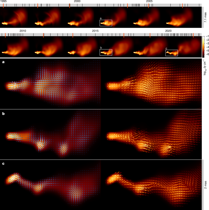
The kine algorithm is a static and dynamic image-reconstruction method designed for very-long-baseline interferometry (VLBI) data. As a forward-modeling imaging technique, it represents the source brightness distribution with a neural field43. This section outlines the kine methodology, beginning with an overview of VLBI measurements and continuing with the neural-field imaging model illustrated in Fig. 4. We then describe the synthetic datasets used to evaluate the algorithm and present the resulting image and video reconstructions. The Supplementary Information includes comprehensive tests of dynamic range, angular resolution, time interpolation and motion tracking, along with a comparison between kine and CLEAN imaging on real observations and details of the optical-flow velocity analysis.
VLBI measurements
In radio interferometry, every antenna in an array records a signal proportional to the electromagnetic flux density received from the sky. According to the van Cittert–Zernike theorem, the time-averaged correlation between signals measured by two antennas—known as a visibility—is the Fourier transform of the source brightness distribution on the sky. This transform is sampled at a spatial frequency determined by the projected separation, or baseline, between the antennas.
For antennas A and B with projected baseline vector \(\bar{b}=({b}_{x},{b}_{y})\), observing at wavelength λ, the ideal complex visibility VAB(u, v, t) is related to the time-dependent flux density distribution \({\mathcal{I}}(x,y,t)\) by
$${V}_{\mathrm{AB}}^{({\mathcal{I}})}(u,v,t)=\int \int \,{{\rm{e}}}^{-2\mathrm{\pi i}(ux+vy)}\,{\mathcal{I}}(x,y,t){\rm{d}}x{\rm{d}}y,$$
(1)
Here, \((u,v)=\left(\frac{{b}_{x}}{\lambda },\frac{{b}_{y}}{\lambda }\right)\) are the spatial frequencies along the x and y directions. A detailed description of radio-interferometric observations and imaging is provided in ref. 44. Although the equation above is written for Stokes \({\mathcal{I}}\), it applies equally to all Stokes visibilities: \(({V}_{\mathrm{AB}}^{({\mathcal{I}})},{V}_{\mathrm{AB}}^{({\mathcal{Q}})},{V}_{\mathrm{AB}}^{({\mathcal{U}})},{V}_{\mathrm{AB}}^{({\mathcal{V}})})\).
In real VLBI observations, visibility measurements are affected by several types of noise and calibration errors. These errors are generally divided into baseline-dependent and station-dependent contributions. The measured visibility can therefore be written as
$${V}_{{\rm{AB}}}^{{\prime} }={G}_{{\rm{A}}}{G}_{{\rm{B}}}{{\rm{e}}}^{{\rm{i}}({\phi }_{{\rm{A}}}-{\phi }_{{\rm{B}}})}({V}_{\mathrm{AB}}+{{\epsilon }}_{\mathrm{AB}}),$$
(2)
In this expression, \({G}_{{\rm{A}},{\rm{B}}}{{\rm{e}}}^{{\rm{i}}{\phi }_{{\rm{A}},{\rm{B}}}}\) represents station-dependent amplitude and phase errors, commonly called complex gains. The term ϵAB denotes thermal noise, which follows a Gaussian distribution with a baseline-dependent standard deviation44. Complex gain errors are particularly challenging because they may be inaccurately estimated during a priori calibration. Thermal noise, in contrast, can be characterized and included in the optimization through the visibility uncertainties σAB.
Although complex visibilities are the primary data product generated by VLBI observations, imaging can also use observables designed to be insensitive to station-based amplitude and phase errors. kine supports complex visibilities VAB, visibility amplitudes |VAB|, closure phases \({\varPhi }_{\mathrm{ABC}}:= \arg ({V}_{\mathrm{AB}}{V}_{\mathrm{BC}}{V}_{\mathrm{CA}})\), closure amplitudes AABCD ≔ |VABVCD/VACVBD| and logarithmic closure amplitudes.
Neural-field model for VLBI imaging
kine is a forward-modeling algorithm for interferometric imaging. It represents a continuous image or time-varying video of the polarized source brightness distribution with a neural field9 parameterized by weights \({\mathcal{W}}\). The neural field uses a coordinate-based multilayer perceptron (MLP)45. The network receives right ascension x, declination y and time t as inputs, and predicts the total intensity, fractional linear polarization, electric-vector position angle and fractional circular polarization at each sky position and time:
$${(\hat{{\mathcal{I}}},{\hat{m}}_{{\ell }},\hat{\chi },{\hat{m}}_{c})}_{{\mathcal{W}}}(x,y,t)={\mathrm{MLP}}_{{\mathcal{W}}}(x,y,t).$$
(3)
The hat symbol identifies estimated quantities rather than the true or directly observed properties of the source. The four Stokes parameters are calculated from the predicted intensity and polarization quantities as follows:
$$\left\{\begin{array}{l}\hat{{\mathcal{I}}}=\hat{{\mathcal{I}}},\\ \hat{{\mathcal{Q}}}=\hat{{\mathcal{I}}}\cdot {\hat{m}}_{{\ell }}\cdot \cos (2\hat{\chi }),\\ \hat{{\mathcal{U}}}=\hat{{\mathcal{I}}}\cdot {\hat{m}}_{{\ell }}\cdot \sin (2\hat{\chi }),\\ \hat{{\mathcal{V}}}=\hat{{\mathcal{I}}}\cdot {\hat{m}}_{c}.\end{array}\right.$$
(4)
The predicted video is passed through a fully differentiable VLBI forward model. The MLP weights are optimized by minimizing a χ2 data-fitting loss between the observed measurements and those predicted by the neural field. Within this model, estimated complex visibilities \(\widehat{V}\) and related interferometric observables are computed by evaluating the two-dimensional Fourier transform of the predicted flux density \(\hat{{\mathcal{I}}}\) at the measured (u, v, t) coordinates.
In practice, \(\hat{{\mathcal{I}}}\) is evaluated on a discrete grid of spatial and temporal coordinates. The visibility calculation therefore uses a discrete Fourier transform, represented by a matrix multiplication. For observation time tj and the ith (u, v) sample, the predicted visibility is
$$\begin{array}{c}{\hat{V}}_{{\mathcal{W}}}({(u,v)}_{i},{t}_{j})=\sum _{k}{{\bf{F}}}_{ik}{\hat{{\mathcal{I}}}}_{{\mathcal{W}}}({(x,y)}_{k},{t}_{j}),\end{array}$$
(5)
The index k covers every spatial coordinate used to represent the video. Both the predicted intensity and the corresponding visibilities depend on the neural-network parameters \({\mathcal{W}}\).
MLP models exhibit a known spectral bias46: gradient-based training tends to learn low spatial frequencies before high spatial frequencies. For VLBI image reconstruction, this behavior provides a useful implicit regularization. It encourages smooth structures and reduces spurious high-frequency features in both the spatial and temporal dimensions. Because the neural representation is continuous, kine can also generate frames at times without direct observations by using correlations learned from neighboring epochs. Similar neural representations have been applied as implicit regularizers in other ill-posed astrophysical imaging problems, where many possible source structures can explain the available measurements47,48,49.
Optimization of the neural-field reconstruction
We formulate VLBI image reconstruction as a noise-weighted data-fitting problem. Assuming Gaussian residuals—which is appropriate for visibilities and amplitudes, and for closure quantities in the high-signal-to-noise regime—the loss function \({\mathcal{L}}\) is the sum of the χ2 contributions from the selected data products:
$${\mathcal{L}}=\sum _{D}{\chi }_{D}^{2}=\sum _{D}\left[\frac{1}{{N}_{t}}\mathop{\sum }\limits_{j=1}^{{N}_{t}}\frac{1}{{k}_{D}{N}_{D,j}}\mathop{\sum }\limits_{i}^{{N}_{D,j}}\frac{{({D}_{ij}-{\hat{D}}_{{\mathcal{W}}ij})}^{2}}{{\sigma }_{D,ij}^{2}}\right],$$
(6)
Here, D denotes a selected data product. The index j runs over the observed times, from 1 to Nt, while i runs over all measurements available at time tj, up to ND,j. The factor kD normalizes each data product according to its degrees of freedom. One or more data-product types can be included in the loss, with the corresponding terms weighted equally.
The optimization repeats three steps until convergence. First, the algorithm evaluates the source video using the current network parameters \({{\mathcal{W}}}_{k}\) on a regular spatial grid, with time coordinates corresponding to the observation epochs. Second, it calculates the loss from the predicted and observed data. Third, it updates the MLP parameters to \({{\mathcal{W}}}_{k+1}\) using gradient descent. Specifically, we use the Adamax optimizer50.
We define convergence as a less-than-1% decrease in the moving average of the loss over 100 iterations for at least 1,000 iterations, provided that every data-product term has reached a value of approximately 1. Convergence typically occurs after about 2 × 10⁴ iterations, which we use as the standard total number of optimization steps.
Calibration-free VLBI imaging
For datasets without gain corruption, complex visibilities are the preferred data product because they preserve the full information content of the observations. In this case, kine simultaneously reconstructs all Stokes parameters during optimization.
When amplitude or phase gains are present, imaging is performed with closure quantities. Closure amplitudes and logarithmic closure amplitudes do not retain the total flux information, so a total-flux regularizer is added to the loss. This term constrains the flux in each frame to a user-specified value or to a value estimated from the instantaneous visibility measured on the shortest baseline.
Closure phases do not preserve the absolute position of the source within the image frame. Consequently, a reconstructed movie may exhibit a smooth apparent drift. We correct this effect after imaging by aligning the frames to a selected feature, such as a jet core. The alignment procedure is described in the Supplementary Information.
The current version of kine does not jointly estimate station gains during imaging. For total-intensity reconstruction, this limitation is addressed by using gain-independent closure quantities. Closure quantities for the \({\mathcal{Q}}\) and \({\mathcal{U}}\) signals are gain-independent only when polarization leakage is absent51. Even under those conditions, the low signal-to-noise ratio of the \({\mathcal{Q}}\) and \({\mathcal{U}}\) measurements, combined with the information loss associated with closure quantities, can leave the data insufficiently constrained.
For this reason, the most effective approach for producing a full-polarimetric video in the presence of gain errors is a three-stage process. First, the data are imaged in total intensity using suitable closure quantities. Second, the measurements are self-calibrated against the total-intensity video reconstruction. Finally, the self-calibrated data are imaged in full Stokes using complex visibilities.
The kine method was developed for reconstructing time-variable sources, but it also supports static VLBI imaging by removing the time coordinate from the network inputs.
Neural-network architecture
kine is implemented in Python with the JAX deep-learning framework52. Total-intensity imaging uses a four-layer MLP, while full-Stokes imaging of self-calibrated data uses a six-layer MLP. Both networks contain 256 nodes per layer and include a residual skip connection53 between the first and final layers.
All hidden-layer outputs, except those of the final layer, are normalized with BatchNorm54 across the complete set of input coordinates to produce zero mean and unit standard deviation. Hidden layers use the Gaussian Error Linear Unit activation function55. The output layer applies SoftPlus to \(\hat{{\mathcal{I}}}\) and sigmoid activations to \({\widehat{m}}_{{\ell }}\), \({\widehat{m}}_{c}\) and \(\widehat{\chi }\).
Standard interferometric operations are provided by the eht-imaging library7. During optimization, spatial coordinates are sampled on a regular grid and time coordinates are taken from the observation timestamps. For the 3C 345 imaging analysis, we used 200 × 200 spatial input points with a spacing of 75 μas.
Computational runtime depends on the number of visibilities and epochs, the ratio between the field of view and synthesized-beam size, and the selected data products. Optimizing the network for 116 VLBA epochs of 3C 345 required approximately 1.3 h on four NVIDIA A100 GPUs. Imaging four days of M 87* EHT observations required approximately 20 min on a single A100 GPU.
Network initialization
When VLBI (u, v)-coverage is sufficiently dense, as in VLBA observations, kine can reconstruct an image or video from randomly initialized network weights. For closure-phase imaging, however, initializing the network with a simple source model, such as a Gaussian, can help place the emission at the correct position in the image frame.
The initialization image should have approximately the correct total flux and cover the region where most of the source emission is expected. The precise shape of the initial model has little effect on the final image or video after convergence.
Initialization is performed by optimizing the network directly against an initial image \({{\mathcal{I}}}_{\mathrm{init}}(x,y)\) with a pixel-to-pixel distance loss:
$${{\mathcal{L}}}_{\mathrm{init}}=\sum _{i,j}{({{\mathcal{I}}}_{\mathrm{init}}({x}_{i},{y}_{i})-{\hat{{\mathcal{I}}}}_{{\mathcal{W}}}({x}_{i},{y}_{i},{t}_{j}))}^{2}$$
(7)
During this step, the image Fourier transform and other interferometric data products are not calculated. Once the network reproduces the initialization image, optimization against the observed data products begins.
Synthetic-data validation
We evaluated kine using several synthetic VLBI datasets designed to match the morphology, coverage and noise characteristics of the real 3C 345 observations. The first ground-truth video, model1, uses a geometric jet whose emission direction precesses along a circular orbit. The jet produces ballistic components that expand and fade as they move away from the core, creating a continuous winding structure.
The second model, model2A, follows a similar prescription but uses greater spacing between emitted components. It therefore consists of distinct features launched at different angles. Each component begins with a full width at half maximum (FWHM) of 80 μas and expands modestly as it moves from the core at an apparent speed of β = 11.4.
The third model, model3A, is based on model2A but adds a parabolic background jet profile to represent a more realistic source structure. We also generated variations to test angular resolution and motion recovery: model2B and model3B use components with FWHM = 60 μas, model2C uses FWHM = 160 μas, model2D uses an apparent speed of β = 22.7 and model2E uses β = 5.7.
For every simulated epoch, we generated synthetic measurements using the corresponding real (u, v)-coverage and the same thermal-noise level as the observations. Complex gain corruption was not added because the closure quantities used during the first imaging stage are invariant to station-based gain errors.
We reconstructed the synthetic datasets with the same settings used for the real observations. Reconstructions of model1, model2A and model3A are presented here as representative examples. The ground-truth videos appear in the first, third and fifth rows of Extended Data Fig. 3, while the corresponding kine reconstructions appear in the second, fourth and sixth rows. The results show that kine reproduces the model structures with high fidelity, as demonstrated by the high average normalized cross-correlation between the true and reconstructed frames in Extended Data Table 1.
The Supplementary Information describes additional tests of dynamic range, super-resolution, component measurements, time interpolation and motion tracking. The resulting image-quality improvements depend on the quantity and quality of the observations and on the available temporal coverage. They should therefore not be interpreted as dataset-independent performance gains.
Forward-modeling imaging methods can achieve higher effective resolution than traditional inverse techniques by incorporating prior information. Our validation tests show that dynamic kine reconstructions achieve effective resolutions of approximately 100–125 μas, with an average of 113 μas. Static reconstructions reach approximately 110–145 μas, with an average of 125 μas. The principal improvement is already present in the static reconstruction, which improves the nominal 475 μas resolution by a factor of 3.8. Dynamic reconstruction provides a further, more modest improvement factor of 4.2.
The higher dynamic range of kine results from improved resolution and the simultaneous reconstruction of multiple epochs. Static reconstructions achieve dynamic ranges between 6 × 10³ and 8 × 10⁴, whereas dynamic reconstructions reach approximately 2 × 10⁵ to 7 × 10⁵. Dynamic imaging therefore delivers an improvement of about one order of magnitude over static imaging, consistent with the expected \(\sqrt{N}=\sqrt{116}\simeq 11\) scaling limit.
To evaluate the recovery of compact features near the core, we fitted double two-dimensional Gaussian models to the kine reconstructions. Components could be accurately located from approximately 110 μas from the core and tracked across their full trajectories. For components fully separated from the core, the position angle was recovered to within 1° of the true value. For components connected to the core, the position angle was recovered to within 7°.
We also tested velocity recovery by combining kine with optical-flow analysis. The results show that apparent velocities in the 3C 345 data can be measured accurately up to at least approximately 23c, exceeding the maximum speeds measured in the real observations.
Because neural fields provide a continuous representation, kine videos can be sampled at arbitrary times rather than only at observed epochs. For data with the coverage and quality of the 3C 345 observations, the method produces reliable, motion-preserving interpolation for frames located up to six months from the nearest observation. We use interpolated frames in the optical-flow analysis to create a regularly sampled video. The largest gap between an interpolated frame and the nearest observation is 5.7 months, within the validated interpolation range.
CLEAN versus kine VLBI imaging
Synthetic-data tests show that, even when individual observations provide sufficient coverage for static imaging, dynamic reconstruction can achieve greater resolution and dynamic range. We therefore measured the effective resolution and dynamic range of static and dynamic kine reconstructions from the real 3C 345 observations and compared them with CLEAN images.
Supplementary Fig. 8 presents a representative comparison between conventional static CLEAN imaging, snapshot static kine imaging and dynamic kine imaging. Both kine reconstructions are consistent with the CLEAN image while revealing substantially more structure in the jet. Because no ground-truth image exists for the real observations, dynamic range is estimated using the conventional definition. Resolution is estimated by comparing power spectra with the CLEAN model convolved with the nominal synthesized beam.
The average dynamic range is 3.6 × 10³ for CLEAN, 4.9 × 10⁴ for static kine and 5.1 × 10⁵ for dynamic kine. These values correspond to an improvement of approximately one order of magnitude for static kine and two orders of magnitude for dynamic kine compared with traditional CLEAN imaging.
Static kine reconstructions show a broad range of dynamic-range values, while dynamic kine produces more consistent results. This indicates that dynamic imaging can improve lower-quality epochs by using information from observations before and after the target epoch.
The measured resolution is 141 μas for static kine and 106 μas for dynamic kine. Relative to CLEAN’s average nominal resolution of 475 μas, set by the diffraction limit, these values represent improvement factors of 3.4 and 4.5, respectively. The results agree with the synthetic-data validation, although the real-data resolution estimates are less certain because they rely on comparison with the CLEAN reconstruction rather than a known ground truth. We therefore use the more conservative synthetic-data estimates for our final conclusions.
Source: www.nature.com