Observations and Data Reduction

We present high-resolution solar observations obtained on 14 April 2025 between 21:38 UT and 21:41 UT with the Daniel K. Inouye Solar Telescope (DKIST)²¹, the world’s largest optical and infrared solar telescope. Atmospheric conditions varied during the observing sequence, although the best periods reached Fried parameter values of approximately \({r}_{0}\approx 12\,\mathrm{cm}\). DKIST’s wavefront-correction system operated in diffraction-limited mode and measured and corrected all optical modes within its detection capabilities.

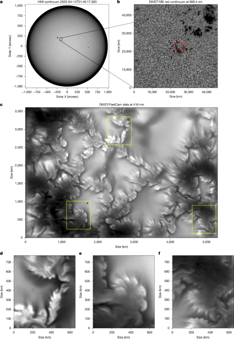
The observations focused on the first target of the day: a pore-containing region near active region NOAA 14060. The target was located close to disk centre at helioprojective Cartesian coordinates of X = −162 arcsec and Y = 168 arcsec, corresponding to \(\mu \approx 0.97\) (Fig. 1).

FastCam High-Resolution Imaging

The primary dataset was acquired with the FastCam diagnostic system at DKIST. This instrument was developed through a collaboration between the National Solar Observatory and the Max Planck Institute for Solar System Research. The system was installed in front of the spectrograph entrance slit of the Visible Spectro-Polarimeter and removed after the diagnostic test.

The optical configuration improved the performance of the Visible Spectro-Polarimeter feed telescope, which otherwise contained no powered optics. Combined with the Max Planck Institute camera’s 5.5 μm pixel-cell size, this arrangement produced a sampling of \(\Delta s\approx 0.00825\,\mathrm{arcsec\,px^{-1}}\), equivalent to approximately 6 km px⁻¹ on the solar surface.

Observations were obtained at 416 nm using a narrowband filter with a full-width at half-maximum of 0.5 nm. The camera read out a 2K × 1K px² region of interest at 740 frames per second, with an exposure time of 100 μs.

The camera included a phase-diversity beam-splitter assembly that simultaneously recorded two images: one in focus and one defocused by approximately 0.4 waves root mean square. These images were projected side-by-side onto the detector in a phase-diversity configuration^38,39. This arrangement enabled us to measure the residual wavefront aberrations remaining after adaptive-optics correction⁴⁰.

The solar field of view common to the focused and defocused images covered approximately 5,800 × 4,350 km² on the Sun, corresponding to 8 × 6 arcsec². The analysed dataset spans approximately 3 min.

FastCam images were reconstructed with multi-frame blind deconvolution⁴¹, which numerically models and removes residual atmospheric aberrations. For each reconstructed science frame, the algorithm processed 2,000 dark- and gain-calibrated camera frames. Following image reconstruction, the effective imaging cadence was 2.7 s.

Most reconstructed frames reached a spatial resolution of approximately 19 km. This value is consistent with the Rayleigh diffraction limit at 416 nm and was inferred from the full-width at half-maximum of the finest structures visible in the observations.

Context Imaging with DKIST/VBI

Context observations were supplied by the Visible Broadband Imager (VBI)⁴². This instrument can acquire large-field, short-exposure image sequences at a single wavelength within 3 s.

For this experiment, the VBI recorded sequences of 80 frames, alternating between the red continuum at 668.4 nm and the Hα line at 656.3 nm; the Hα data are not shown here. The images had a sampling of 12.3 km px⁻¹, or 0.017 arcsec px⁻¹.

Each consecutive image sequence was reconstructed with speckle-reconstruction algorithms⁴³ to reduce residual seeing effects across the large field of view, which covered approximately 50 × 50 Mm², or 69 × 69 arcsec².

The VBI red channel began recording 3 min after the FastCam observations. Nevertheless, its field of view clearly contained the evolved structure corresponding to the higher-resolution FastCam dataset (Fig. 1).

Full-Disk Context from SDO/HMI

Full-disk observations were obtained with the Helioseismic and Magnetic Imager onboard NASA’s Solar Dynamics Observatory (SDO/HMI)⁴⁴. Figure 1a presents an HMI photospheric continuum image recorded at 21:40 UT.

The HMI image was coaligned with the DKIST/VBI/FastCam observations using the SolarSoft auto_align_images function and a cross-correlation procedure (Fig. 1).

Numerical Simulations and Spectral Synthesis

We compared the observations with magnetohydrodynamic (MHD) simulations calculated using the MURaM code²². To achieve very high spatial resolution, we modelled a compact domain measuring 6.144 × 6.144 × 2.048 Mm³. The vertical coordinate was denoted by \(z\), and the domain was comparable in size to the high-resolution FastCam field of view.

The vertical extent reached approximately 1.367 Mm below \(z=0\) Mm and 0.681 Mm into the overlying atmosphere. Including the stable atmosphere above the photosphere was essential because a solar-like configuration driven by radiative losses could not be established without it. This realistic photospheric structure provided the necessary connection between the numerical model and the DKIST observations.

We began with a relaxed hydrodynamic simulation and added a vertical magnetic-field component derived from the HMI magnetogram of the observed region (Supplementary Fig. 1). The initial magnetic field had the form \(n{B}_{z}-(n-1)\langle {B}_{z}\rangle\), where \({B}_{z}\) was taken from the HMI magnetogram and amplified to compensate for magnetic-field dispersal caused by granular motions during a further relaxation period of approximately 1.8 h. Here, \(n\) denotes the enhancement factor.

After relaxation, the individual magnetic-flux concentrations were no longer influenced by the initial configuration. The key parameter for realistic magnetoconvection is the net magnetic-flux imbalance, which remained unchanged by the enhancement. Therefore, the amplified HMI magnetogram was used only to create an initial distribution resembling the observations; it was not required for the development or investigation of Kelvin–Helmholtz instabilities (KHIs).

We found that \(n=2.5\) produced a large-scale magnetic-field distribution comparable to the HMI magnetogram and generated pores resembling those observed (Supplementary Fig. 1). Following initialization, the simulation evolved for 4,980 s with a grid spacing of 12.8 km, followed by 1,200 s at 6.4 km and a further 1,200 s at 3.2 km.

The analysed sequence corresponds to 480–720 s within the 3.2-km simulation phase, or 5,460–5,700 s after initialization with the HMI magnetogram. The simulation used 12 opacity bins and the Asplund 2009 opacities⁴⁵.

The 3.2-km grid spacing exceeded the expected photospheric diffusive length scale of approximately 1.4 km. This estimate follows from the Spitzer diffusivity \(\eta=2\times10^{8}\,\mathrm{cm^{2}\,s^{-1}}\) and a characteristic timescale of \(\tau=100\) s, using \(l\approx\sqrt{\eta\tau}\)⁴⁶. The numerical diffusivity implemented in MURaM²² is therefore justified for the simulations presented here. Higher-resolution calculations, however, would require a spatially dependent Spitzer diffusivity.

Synthetic Spectra and Filtergrams

Developed simulation snapshots were used to calculate synthetic spectra over the wavelength interval 415.32–416.7 nm. The calculations included 500 spectral points and used the one-dimensional Rybicki–Hummer radiative-transfer code⁴⁷ under the assumption of local thermodynamic equilibrium (Extended Data Fig. 4c).

The spectral synthesis included molecular CH and CN features, atomic lines and the continuum within the observed filter bandpass. Intensities were also calculated at a single continuum wavelength of 500 nm. To reduce computational requirements, the vertical grid was downsampled to 9.6 km by retaining every third grid point along the vertical axis.

Spectra were synthesized at disk centre and near the solar limb, corresponding to \(\mu=1\) and \(\mu=0.97\), respectively. For the \(\mu=0.97\) calculations, each horizontal layer of the MURaM cube was shifted relative to the layer below by \(\Delta z\,\tan(\theta)\), where \(\Delta z\) is the vertical grid spacing and \(\theta\) is the heliocentric angle between the line of sight and the solar-surface normal. This transformation aligned the inclined line of sight with the vertical direction.

For the \(\mu=0.97\) data, pixel sampling was foreshortened along the \(y\) direction by a factor of \(\mu\) and increased along the \(z\) direction by \(1/\mu\). To reproduce the DKIST 416-nm filtergrams, the synthetic intensities were multiplied by the transmission profile of the diagnostic interference filter (Extended Data Fig. 4c) and integrated over the wavelength interval covered by the filter.

Extended Data Fig. 4a,b shows that the synthetic images reproduced the principal features seen in the 416-nm observations, including KHI vortices and striations. Extended Data Fig. 4c compares the synthetic spectrum averaged across the simulation field of view with a solar atlas⁴⁸ observed over the same wavelength range using a Fourier-transform spectrometer. The close agreement between the two spectra demonstrates that the simulation reproduced the observed spectral features with high accuracy.

The agreement between the synthetic and observed spectra and images confirms that the MURaM simulations provide an effective diagnostic framework for interpreting high-resolution 416-nm solar-intensity observations.

Formation Heights and Photospheric Striations

Using the MURaM snapshot, we calculated the geometrical height at which the optical depth reached unity for different wavelengths across the synthesized spectral interval (Extended Data Fig. 9k,l). The heights of \(\tau=1\) and \({\tau}_{415.91}=1\), together with those of other 416-nm continuum wavelengths, were nearly identical, differing only marginally. This result indicates that the continuum wavebands near 416 nm formed at approximately the same geometrical heights.

We used the optical depth at 500 nm to identify the heights at which KHI properties were directly measured in the MURaM cube and compared with the synthetic 416-nm filtergrams.

Striations have traditionally been observed and studied mainly at inclined viewing angles^27–30. Our simulations demonstrate that these structures are also present at disk centre. Extended Data Fig. 9k shows that the features visible in the disk-centre filtergrams result from opacity variations.

Their emergent intensity is strongly correlated with spatial variations in \({B}_{z}\) and anticorrelated with density in the layers above the KHI formation heights (Supplementary Fig. 9). These variations shift the geometrical height at which the emergent intensity forms, producing striation-like patterns in the disk-centre synthetic filtergrams.

This mechanism is equivalent to the process responsible for striations at inclined viewing angles^28–31. Inclined viewing makes the structures appear longer and more extended toward the limb, which improves their detectability. However, our results indicate that striations should also be detectable at disk centre when observations achieve sufficiently high spatial resolution.

KHI Growth Rate in Linear MHD Theory

Linear MHD theory predicts that the Kelvin–Helmholtz instability grows most rapidly when the shear flow is perpendicular to the magnetic field and the wavevector is aligned with the shear velocity²³. For finite, continuous velocity profiles, the fastest-growing wavelengths depend on the thickness of the velocity-shear layer.

Chandrasekhar²³ examined the KHI in a slab geometry consisting of two adjacent incompressible fluids with different densities, separated by a finite-width shear layer of intermediate density. Within the shear layer, the velocity changes linearly from \(-{U}_{0}\) to \(+{U}_{0}\) across a distance \(d\). The velocity and density profiles are given by equation (1) (Supplementary Fig. 10):

Here, \({\rho}_{0}\) is the density within the shear layer, \(\epsilon\) defines the density contrast between the two surrounding layers, \(x\) is the coordinate across the KHI interface and \(d\) is the thickness of the velocity-shear layer.

Continuity of the perturbation equations leads to the following dispersion relation²³:

In this expression, \(\nu=\gamma/k{U}_{0}\), \(\kappa=kd\), \(\gamma\) is the frequency and \(k\) is the KHI wavenumber. Magnetic-field effects and the Richardson number are neglected because the shear flow is perpendicular to the magnetic field and the wavevector is perpendicular to gravity.

Equation (2) is a transcendental equation for the complex frequency \(\gamma={\gamma}_{\rm r}-{\rm i}{\gamma}_{\rm im}\). The imaginary component, \({\gamma}_{\rm im}\), describes the instability and determines the exponential growth rate of unstable modes. The real component, \({\gamma}_{\rm r}\), gives the frequency and is related to the phase speed \(v_{\rm ph}\) of the KHI modes through \({\gamma}_{\rm r}=k{v}_{\rm ph}\).

Extended Data Fig. 6 illustrates how the KHI wavelength, growth rate and phase speed depend on \({U}_{0}\), \(d\) and \(\epsilon\) over the parameter ranges measured in the observations and simulations (Extended Data Table 1).

Estimating KHI Parameters

We estimated the KHI growth rate and phase speed by measuring the relevant physical parameters in both the MURaM simulations and the observations. Several prominent examples are summarized in Extended Data Table 1.

The simulations show that the KHI develops coherently across multiple horizontal layers. Figure 4, Extended Data Fig. 9 and Supplementary Video 5 demonstrate that KHI vortices are three-dimensional structures whose amplitudes vary with height.

The KHI patterns visible in the 416-nm filtergrams are primarily determined by the layer where the continuum optical depth at 416 nm, or 500 nm, approaches unity. Because of the Wilson depression, the \(\tau=1\) layer occurs at different geometrical heights inside and outside the magnetic-flux concentrations (MFCs) (Extended Data Fig. 9). We therefore measured the KHI parameters at the height where the average continuum optical depth at 500 nm reached unity.

First, we identified the KHI interface at this height and calculated the component of the two-dimensional velocity vector parallel to the interface, \({v}_{\parallel}\). We then determined the average one-dimensional velocity profile perpendicular to the interface (Extended Data Fig. 7f and Supplementary Figs. 3f–6f).

The mean thickness of the velocity-shear layer was defined as the spatial region over which the parallel velocity component transitioned between the two surrounding layers. The shear velocity, \(\Delta U\), was estimated from the difference in \({v}_{\parallel}\) across the shear layer using a linear fit to the velocity profile (Extended Data Fig. 7f and Supplementary Figs. 3f–6f).

We also determined the mean densities on both sides of the shear layer along cuts perpendicular to the KHI surface. The wavelength \(\lambda\) was measured as the separation between adjacent developing vortices during the initial, linear-growth phase of the instability (Extended Data Figs. 2c and 5c).

The KHI growth rate was determined from the temporal evolution of the instability amplitude. During the linear phase, the perturbation amplitude increases exponentially, \(A\)