Aberrant Excitatory Neuronal ERBB4 Drives Alzheimer’s Disease Pathology

Mice and Alzheimer’s Disease Mouse Models

All mouse experiments were conducted under protocols approved by the Institutional Animal Care and Use Committees (IACUC) of the Korea Advanced Institute of Science and Technology (KAIST) and the Institute for Basic Science (IBS). Experiments followed applicable animal welfare and ethical guidelines. B6.Cg-Tg(APPswe, PSEN1dE9)85Dbo/Mmjax (APP/PS1) mice and B6.Cg-Tg(APPSwFlLon, PSEN1*M146L*L286V)6799Vas/Mmjax (5×FAD) mice were generated in our laboratory and maintained by breeding with C57BL/6J mice. Mice were housed under a 12 h–12 h light–dark cycle. Both male and female mice were used unless otherwise indicated in the figure legends. Animals were randomly assigned to experimental groups, and all experiments were conducted by investigators blinded to the experimental conditions. Sex was not considered as a biological variable unless specifically stated in the figure legends.

Human Brain Tissue Sections

Human formalin-fixed, paraffin-embedded (FFPE) brain tissue sections were provided by the SNUH Brain Bank. The use of these sections was reviewed and determined to be exempt from review by the Public Institutional Review Board designated by the Ministry of Health and Welfare of the Republic of Korea. All experiments involving human-derived materials were performed in accordance with applicable regulations and institutional requirements.

Cell Lines for AAV Production

HEK293T cells obtained from the American Type Culture Collection (ATCC) were used exclusively for adeno-associated virus (AAV) production. Cells were maintained in our laboratory and were not independently authenticated for this study. HEK293T cultures were confirmed to be free of mycoplasma contamination.

Antibodies and Experimental Reagents

The primary antibodies and working dilution factors were as follows: anti-S100β (Abcam, ab52642; Synaptic System, 287-004; Aves Labs, S100B-0020; 1:500), anti-IBA1 (Wako, 019-19741; Novus, NB100-1028; 1:500), anti-mCherry (Invitrogen, M11217; Aves Labs, mCherry-0020; 1:1,000), anti-vGLUT1 (Millipore, AB5905; 1:1,000), anti-PSD95 (Invitrogen, 51-6900; 1:500), anti-vGAT (Synaptic System, 131-004; 1:1,000), anti-gephyrin (Synaptic System, 147-008; 1:500), anti-FOS (Cell Signaling, 2250S; Synaptic System, 226-308; Synaptic System, 226-017; 1:500), anti-MEGF10 (Merck, ABC10; 1:500), anti-ERBB4 (Abcam, ab32375; Cell Signaling, 4795T; 1:500), anti-parvalbumin (Swant, GP72; 1:1,000), anti-beta amyloid (BioLegend, 803001; Cell Signaling, 2454S; 1:1,000), anti-GFAP (Abcam, ab4674; 1:1,000), anti-AXL (R&D Systems, AF854; 1:100), anti-somatostatin (BMA Biomedicals, T-4103; 1:500), anti-VIP (Synaptic System, 443-005; 1:500), anti-NeuN (Sigma-Aldrich, ABN91; 1:500), anti-cleaved caspase-3 (Cell Signaling, 9661S; 1:500), anti-TREM2 (R&D Systems, AF1729; 1:500), anti-HA (Cell Signaling, 3724S; 1:500) and anti-pS6 (Cell Signaling, 2211S; 1:500).

The secondary antibodies included donkey anti-goat IgG (H&L) Alexa Fluor 405 (Abcam, ab175665), donkey anti-goat IgG (H+L) Alexa Fluor 488 (Jackson Laboratory, 705-545-003), donkey anti-chicken DyLight 405-conjugated AffiniPure, donkey anti-chicken IgY (IgG) (H+L) (Jackson Laboratory, 703-475-155), donkey anti-chicken IgG (H+L) Alexa Fluor 488 (Jackson Laboratory, 703-545-155), donkey anti-chicken IgG (H+L) Alexa Fluor 594 (Jackson Laboratory, 709-585-155), donkey anti-rat IgG (H+L) Alexa Fluor 594 (Invitrogen, A-21209), donkey anti-rat IgG (H&L) Alexa Fluor 647 (Abcam, ab150155), donkey anti-rabbit IgG (H&L) Alexa Fluor 405 (Abcam, ab175649), donkey anti-rabbit IgG (H+L) Alexa Fluor 488 (Invitrogen, A-21206), donkey anti-rabbit IgG (H+L) Alexa Fluor 594 (Invitrogen, A-21207), donkey anti-guinea pig IgG (H+L) Alexa Fluor 488 (Jackson Laboratory, 706-545-148), donkey anti-guinea pig IgG (H+L) Alexa Fluor 594 (Jackson Laboratory, 706-585-148), donkey anti-guinea pig IgG (H+L) Alexa Fluor 647 (Jackson Laboratory, 706-605-148), donkey anti-sheep IgG H&L Alexa Fluor 488 (Abcam, ab150177) and donkey anti-mouse IgG (H+L) highly cross-adsorbed secondary antibody Alexa Fluor 594 (Invitrogen, A-21203). Alexa Fluor 488-conjugated secondary antibodies were used at 1:1,000, and all other secondary antibodies were used at 1:500. Additional reagents included HistoVT One (Nacalai, 06380-05) and clozapine N-oxide (CNO; Sigma-Aldrich, C0832-5mg).

Python Packages for Genomic and Statistical Data Analysis

Data analysis used Python v.3.10.0 and the following packages: numpy v.2.0.2, pandas v.2.2.3, matplotlib v.3.9.2, collections (a built-in Python module), scanpy v.1.10.4, scvi v.1.3.0, gseapy v.1.1.8, semopy v.2.3.11, pyWGCNA v.2.2.1, statsmodels v.0.14.5, scipy v.1.15.2, scikit-learn v.1.6.1 and magic-impute v.3.0.0.

Single-Nucleus RNA Sequencing and Bioinformatics Analysis

Single-nucleus RNA sequencing (snRNA-seq) data were processed using Cell Ranger v.8.0.1. Briefly, raw BCL files generated on an Illumina HiSeq platform were demultiplexed into FASTQ files with ‘cellranger mkfastq’. FASTQ files were processed with ‘cellranger count’, including alignment to the mouse reference genome mm10-2020-A, gene-expression quantification based on unique molecular identifiers and cell barcodes, cell clustering and differential gene-expression analysis. Data from multiple sequencing runs were integrated using cellranger aggr.

Raw 10x Genomics count matrices were imported into Scanpy v.1.10.4. Genes detected in at least 3 cells and cells containing 200–8,000 detected genes were retained for downstream analysis. Cells with mitochondrial gene content exceeding 5% were removed. Doublets were identified and excluded using scanpy.pp.scrublet with default settings. After quality-control filtering, count data were normalized using Pearson normalization. Highly variable genes were identified with scanpy.experimental.pp.normalize_pearson_residuals and scanpy.experimental.pp.highly_variable_genes, respectively. SysVI integration was then performed using approximately 3,000 highly variable genes and the package tutorial (https://docs.scvi-tools.org/en/stable/tutorials/notebooks/scrna/sysVI.html). Integrations involving all cell clusters used 100–200 epochs, whereas integrations focused on individual cell types, including excitatory neurons, astrocytes or microglia, used 5–30 epochs to achieve the minimum reconstruction loss between the training and validation sets. Clustering and UMAP dimensionality-reduction analyses were performed using the default settings for scanpy.tl.leiden and scanpy.tl.umap. Differentially expressed genes (DEGs) were identified with scanpy.tl.rank_genes_groups using the Wilcoxon rank-sum test and filtered according to adjusted P values and log-transformed expression fold changes. Weighted gene co-expression network analysis (WGCNA) was performed in Python with pyWGCNA v.2.2.1, following the published vignettes (https://github.com/mortazavilab/PyWGCNA/blob/main/tutorials/Quick_Start.ipynb). Gene set enrichment analysis (GSEA) was performed with gseapy v.1.1.8 according to the online tutorial (https://gseapy.readthedocs.io/en/latest/introduction.html). Square-root-transformed normalized counts, calculated using numpy.sqrt(scanpy.pp.normalize_total(anndata, inplace=False)[‘X’]), were used for dot plots, UMAP visualizations and DEG analysis. Magic-imputed counts⁵⁵ were used to visualize violin plots, following the relevant documentation (https://magic.readthedocs.io/en/stable/tutorial.html).

Numbers of Cells Analysed

The numbers of cells analysed were as follows: Fig. 2a included 23,217 cells from 3-month-old wild-type (WT) mice, 22,718 cells from 2-month-old 5×FAD mice and 33,623 cells from 3-month-old 5×FAD mice. Fig. 2b included 9,069 excitatory neurons from 3-month-old WT mice, 10,231 excitatory neurons from 2-month-old 5×FAD mice and 14,044 excitatory neurons from 3-month-old 5×FAD mice. Hippocampal samples in each group were obtained from two mice.

Figure 5a included 6,763 sgControl and 12,826 sgErbb4 excitatory neurons; Fig. 5b included 3,199 sgControl and 2,840 sgErbb4 microglia; and Fig. 5c included 729 sgControl and 1,436 sgErbb4 astrocytes. Figure 5i included 8,570 HA and 10,442 Erbb4 excitatory neurons; Fig. 5j included 1,037 HA and 1,450 Erbb4 microglia; and Fig. 5k included 1,857 HA and 1,267 Erbb4 astrocytes. For each comparison, cells were obtained from three mice per group.

Stereotaxic AAV Injection and Brain Transduction

All AAVs were produced in our laboratory as previously described⁷. Briefly, pAAV9 capsid plasmid, helper plasmid for viral assembly and target plasmids were co-transfected into HEK293T cells obtained from the Korean Cell Line Bank using a polyethyleneimine (PEI)-based transfection method at 0.3 mg ml⁻¹⁵⁶. HEK293T cells were cultured in fetal bovine serum (FBS)-containing Dulbecco’s modified Eagle’s medium (DMEM; Welgene, with FBS from Gibco). The medium was replaced with serum-free medium during transfection for 6–12 h. Transfected cells were incubated at 37 °C in a humidified incubator containing 5% CO₂. After 72 h, the culture medium was collected and replaced with fresh medium. The collected medium was stored at 4 °C. After an additional 48 h, both the medium and HEK293T cells were harvested and purified using a polyethylene-glycol-mediated method⁵⁷. Purified AAV preparations were concentrated to 200 μl using a 100 kDa Amicon Ultra centrifugal filter tube (Millipore).

For sgRNA-mediated targeting of Erbb4, the sequence TTAGCGATATTCTTAAACTA was cloned into the SaCas9 vector. The sequence GGTCGGGGCGTATGCGTCTA was also cloned into the SaCas9 vector. For sgRNA-mediated targeting of Rptor, the sequence TGCAGGTCGTATATGGACAG⁵⁸ was cloned into the SaCas9 vector. The control sgRNA was a non-targeting sequence with no predicted target sites in the mouse genome, based on previously reported screening data⁵⁹. For Erbb4 overexpression, Erbb4 cDNA was purchased from Sino Biological (MG51064) and cloned into an AAV target vector. The kinase-dead Erbb4 mutant was generated by manually substituting methionine for lysine at position 751. Control shRNAs were CATTGCTGGCACGAAGATTGAC and GTAGCAGAGCACCGTTTACATG. shRNAs targeting Megf10 were TGAATCTTAAAAATGTGAATCC and GTTATTACAGAACCTAAGTGA.

Stereotaxic AAV injections into the mouse brain were performed as previously described^7,37. Mice were anaesthetized with isoflurane (Piramal) delivered using a veterinary vaporizer (Surgivet). The head was disinfected with 70% ethanol, the hair was removed and a skin incision was made. For ExPre and chemogenetic experiments using the hSyn promoter, AAVs were injected into CA3 at the following coordinates: mediolateral (ML), −2.5 mm; anteroposterior (AP), −2.0 mm from bregma; dorsoventral (DV), −2.2 mm from the brain surface. For InhiPre, chemogenetic experiments using the Gad67 promoter, SaCas9 with sgRNAs, shRNA experiments, Erbb4 overexpression and oligomeric Aβ injections, AAVs were delivered to CA1 at ML, −1.25 mm; AP, −2.0 mm from bregma; and DV, −1.5 mm from the brain surface. Bilateral viral injections were used only for behavioural experiments. Mice receiving oligomeric Aβ were euthanized 2 days after injection. Mice in the Erbb4 overexpression experiments were euthanized 2 weeks after injection. For all other AAV-mediated experiments, mice were euthanized 3 weeks after injection unless otherwise indicated in the figure legend. For chemogenetic experiments, CNO was administered at 0.5 mg kg⁻¹ for 4 consecutive days before euthanasia. The same viral titre was used for each cohort. Following injection, the incision was closed using Reflex 7 mm wound clips (ROBOZ).

Immunohistochemistry, FISH, Antigen Retrieval and Confocal Image Analysis

Mice were anaesthetized with avertin at 20 μl g⁻¹ by intraperitoneal injection and transcardially perfused with 1× PBS (Welgene), followed by 4% paraformaldehyde (PFA). Brains were post-fixed overnight in 4% PFA at 4 °C and then transferred to 30% sucrose in 1× PBS for 48 h. Tissue was embedded in OCT compound (Leica) and sectioned into 30 μm coronal slices using a cryostat microtome (Leica). Sections were permeabilized and blocked for 1 h at room temperature in buffer containing 4% BSA and 0.3% Triton X-100 in 1× PBS. Sections were incubated with the appropriate primary antibodies for 24 h at 4 °C, washed with PBST containing 0.1% Tween-20 in 1× PBS and incubated with the appropriate Alexa Fluor-conjugated secondary antibodies (Invitrogen, Abcam or Jackson ImmunoResearch) in PBST for 2 h at room temperature. After washing, sections were mounted on glass slides. Lipofuscin autofluorescence was reduced by applying TrueBlack (Biotium), diluted 1:20 in 70% ethanol, for 2 min at room temperature. Sections were washed with distilled water and mounted using Vectashield with or without DAPI (Vector Laboratories). Samples were stored at 4 °C until confocal imaging.

For ERBB4 immunohistochemistry, antigen retrieval was performed before the standard staining procedure. Tissue slices were placed in an Eppendorf tube containing 500 μl of 1× HistoVT One solution and incubated at 70 °C for 20 min. Sections were then transferred to a 24-well plate for conventional immunohistochemistry.

For fluorescence in situ hybridization (FISH), tissue sections were cut to 10 μm and mounted on SuperFrost Plus glass slides (Thermo Fisher Scientific). Sections were fixed in 4 °C PFA for 15 min and dehydrated at room temperature through a graded ethanol series consisting of 50%, 70%, 100% and 100% ethanol for 5 min at each concentration. Human FFPE sections were deparaffinized before following the same RNAscope workflow. After air-drying, FISH was performed using RNAscope Multiplex Fluorescent Assay kits (Advanced Cell Diagnostics) according to the manufacturer’s instructions, with minor modifications. Sections underwent protease treatment for 30 min and were then hybridized with target-specific RNAscope probes. Hybridization, amplification and washing steps were performed manually at room temperature or at the temperatures specified by the manufacturer. Signals were detected using Opal TSA fluorophores (Akoya Biosciences) diluted 1:1,000 according to probe and channel requirements. Nuclei were counterstained with DAPI.

Confocal images of brain sections were acquired using a Zeiss LSM880 confocal laser-scanning microscope with ×10, ×20 or ×40 oil-immersion objectives for quantitative analysis as described below. Unless otherwise indicated in the figure legends, data represent measurements from mice.

To measure Erbb4 mRNA levels in mouse pyramidal neurons, single-plane confocal images showing Gad1 and Erbb4 signals in the pyramidal layer were isolated. Colocalization between Gad1 and Erbb4 was quantified using the DiAna plugin. Areas of colocalization were subtracted from the total Erbb4⁺ area to exclude Erbb4 mRNA originating from Gad1⁺ inhibitory neurons.

To quantify ERBB4 mRNA in excitatory neurons from human tissue, single-plane confocal images containing ERBB4, SLC17A7 and DAPI signals were analysed. SLC17A7⁺ excitatory neurons were identified by the presence of SLC17A7 puncta within DAPI⁺ nuclei. ERBB4 puncta colocalized with the SLC17A7⁺DAPI⁺ signal were measured using the DiAna⁶⁰ plugin.

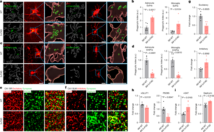
To quantify synapse phagocytosis by glial cells, single-plane confocal images were separated into GFP intensity subtracted from mCherry intensity, representing mCherry-only signal, and glial-cell markers S100β and IBA1. The colocalized area that was mCherry-only⁺ and glial-cell⁺ was measured using the DiAna⁶⁰ plugin. To account for differences in viral delivery, colocalization areas were normalized to GFP-positive areas.

To quantify excitatory and inhibitory synapse numbers, single-plane confocal images of excitatory synaptic markers vGLUT1 and PSD95, and inhibitory synaptic markers vGAT and gephyrin, were analysed separately. Marker areas were measured using the Analyze Particles function in ImageJ, and colocalized areas were quantified using the DiAna plugin.

To quantify GFAP, S100β, IBA1 and beta-amyloid (Aβ) areas, single-plane confocal images of each marker were isolated and analysed using the Analyze Particles function in ImageJ.

To quantify pS6-positive areas in pyramidal neurons and PV⁺ neurons, single-plane confocal images showing pS6, PV and NeuN were isolated. Colocalization of pS6⁺PV⁺NeuN⁺ or pS6⁺PV⁻NeuN⁺ signals was measured using the DiAna plugin.

To quantify the disease-associated microglia (DAM) population, defined by AXL⁺/TREM2⁺ expression, single-plane confocal images of AXL, TREM2 and IBA1 were isolated. AXL⁺IBA1⁺ and TREM2⁺IBA1⁺ colocalization was quantified using the DiAna plugin.

To measure MEGF10 in shRNA-treated samples, single-plane confocal images of MEGF10 and TagBFP were isolated separately, and their colocalized areas were measured with the DiAna plugin. Colocalization areas were normalized to TagBFP-positive areas to account for differences in labelled astrocyte numbers.

To quantify cleaved caspase-3⁺, FOS⁺ or ERBB4⁺ neurons, confocal z-stack images containing cleaved caspase-3, FOS or ERBB4 together with neuronal markers were merged. PV, SST or VIP and NeuN signals were used to identify neurons, and positive cells were counted manually.

Hippocampal Slice Electrophysiology

Mice were anaesthetized with isoflurane and decapitated. Brains were rapidly removed and transferred to ice-cold artificial cerebrospinal fluid (ACSF) continuously bubbled with 95% O₂ and 5% CO₂. ACSF contained 125 mM NaCl, 2.5 mM KCl, 1.25 mM NaH₂PO₄, 25 mM NaHCO₃, 1 mM MgCl₂, 2 mM CaCl₂ and 15 mM glucose. Coronal slices were prepared in ice-cold ACSF using a vibratome (VT1200S, Leica). Slices recovered in ACSF at 34 °C for 20 min and were then incubated at room temperature for at least 40 min. For recording, slices were transferred to a submerged chamber and continuously perfused with oxygenated ACSF at 2–3 ml min⁻¹. The chamber temperature was maintained at 30–31 °C, and recordings were completed within 4–5 h of recovery. Neurons were visualized using infrared differential interference contrast microscopy with an upright microscope (BX51WI, Olympus). Whole-cell voltage-clamp recordings were performed with borosilicate glass pipettes having a resistance of 2.5–3.5 MΩ. Pipettes were filled with a Cs⁺-based low-Cl⁻ internal solution containing 135 mM CsMeSO₃, 10 mM HEPES, 1 mM EGTA, 3.3 mM QX-314, 0.1 mM CaCl₂, 4 mM Mg-ATP, 0.3 mM Na₃-GTP and 8 mM Na₂-phosphocreatine. The solution was adjusted to pH 7.3 with CsOH and had an osmolarity of 290–300 mOsm. Recordings were included only when access resistance was 10–20 MΩ and remained stable, with less than 20% variation throughout the experiment. Whole-cell recordings were acquired using a Multiclamp 700B amplifier (Molecular Devices), filtered at 2 kHz and digitized at 10 kHz using an NI PCIe-6259 data-acquisition device (National Instruments). Data were monitored and acquired with WinWCP (Strathclyde Software) and analysed using Clampfit v.10.7 (Molecular Devices) and OriginPro 2017 (OriginLab). To record miniature excitatory and inhibitory postsynaptic currents (mEPSCs and mIPSCs), tetrodotoxin (TTX; 500 nM; Alomone Labs, T-550) and the NMDA receptor antagonist D-AP5 (25 μM; Tocris, 0106) were added to the ACSF throughout recording. mEPSCs and mIPSCs were recorded sequentially from the same cell. mEPSCs were recorded at −70 mV, the reversal potential for chloride, and mIPSCs were subsequently recorded at 0 mV, the reversal potential for ionotropic glutamate receptors. Each recording lasted 3 min. The full 3 min period was analysed for mEPSCs, whereas mIPSCs were analysed during a 60 s segment beginning 60 s after recording onset.

For intrinsic excitability measurements, 300 μm coronal slices containing the dorsal hippocampal CA1 region were prepared in ice-cold, oxygenated sucrose-based cutting solution containing 75 mM sucrose, 76 mM NaCl, 2.5 mM KCl, 25 mM NaHCO₃, 25 mM glucose, 1.25 mM NaH₂PO₄, 7 mM MgSO₄ and 0.5 mM CaCl₂. The solution was equilibrated with 95% O₂ and 5% CO₂ and adjusted to pH 7.3. Slices were recovered in the same solution for 30 min at 32 °C. They were then transferred to an incubation chamber containing oxygenated ACSF with 124 mM NaCl, 2.5 mM KCl, 1.3 mM MgCl₂, 2.5 mM CaCl₂, 1.0 mM NaH₂PO₄, 26.2 mM NaHCO₃ and 20 mM glucose. The ACSF was adjusted to pH 7.4, and slices were maintained at room temperature for less than 6 h before recording.

For patch-clamp experiments, slices were transferred to a recording chamber perfused with oxygenated ACSF at 30–32 °C using a peristaltic pump. Patch electrodes were pulled from borosilicate glass (Harvard Apparatus, 30-0065) with a micropipette puller (Narishige, PC-10). Electrode resistance was 5.0–7.0 MΩ. Signals were recorded with a Multiclamp 700B amplifier and digitized using a Digidata 1550 digitizer (Molecular Devices) and Clampex software. Signals were amplified, filtered at 2 kHz and sampled at 10 kHz.

For current-clamp recordings, the membrane potential was held at −70 mV using an intracellular solution containing 135 mM K-gluconate, 7 mM NaCl, 10 mM HEPES, 0.5 mM EGTA, 2 mM Mg-ATP, 0.3 mM Na₂-GTP and 10 mM Na-phosphocreatine. The solution was adjusted to pH 7.3 and 295 mOsm. Current-clamp recordings began 5 min after establishing whole-cell configuration. Intrinsic excitability was assessed by injecting 500 ms depolarizing currents from −200 to 500 pA in 50 pA increments. Mean firing rate was calculated from the number of evoked action potentials produced by each current injection. Input resistance (R_in) was estimated from the slope of the I–V relationship, calculated from the difference between baseline and steady-state membrane potentials.

Mouse Behavioural Tests

Novel-object recognition and novel-object location tests were performed in a custom-made square acrylic box measuring 30 cm × 30 cm × 28 cm (W × D × H). One side of the box contained a stripe to provide spatial-location information. Both behavioural paradigms consisted of habituation, training and testing phases.

For the novel-object location test, mice were habituated by freely exploring the open-field arena for 10 min. Twenty-four hours later, mice were placed in the box containing two identical objects for a 10 min training session. After a further 24 h, mice were returned to the box for 10 min, with one object moved to a new location.

For the novel-object recognition test, mice underwent the same habituation procedure. During training, mice were exposed to two identical objects. During testing, one object was replaced with a novel object.

For the spontaneous-alternation test, mice were placed in the centre of a Y-maze. Each arm of the custom-made acrylic maze measured 5 cm × 30 cm × 15 cm (W × D × H), and mice were allowed to explore for 8 min.

For the novel-object location and novel-object recognition tests, the time spent interacting with the familiar and novel objects or locations was measured. The discrimination index was calculated using the following equation:

For spontaneous alternation, entries into all maze arms were recorded and the alternation percentage was calculated using the following equation:

Spontaneous alternation was defined as sequential entry into all three arms of the Y-maze.

The Barnes maze was conducted using the shortened protocol described previously⁴¹. The maze consisted of a circular white platform 1 m in diameter, elevated approximately 1 m above the floor, with 20 evenly spaced perimeter holes. One hole provided access to a dark escape cage. The protocol comprised habituation, training and probe phases. During habituation, mice were placed in the centre of the maze for 30 s and then gently guided to the target hole to familiarize them with the escape cage. During training, mice were placed inside a transparent cylinder at the centre of the maze for 10 s. The cylinder was then removed, and mice were allowed up to 2 min per trial to locate the target hole. Training comprised five trials over 2 days, with three trials on day 1 and two trials on day 2 and an inter-trial interval of approximately 20 min. Mice that did not enter the escape cage within the time limit were gently guided to the target hole. Primary latency, defined as the time from trial onset to the first nose poke at the target hole, was used as a measure of spatial learning. One day after the final training session, a 2 min probe trial was performed with the escape cage removed. The time spent in each quadrant was recorded as a measure of spatial memory.

All behavioural experiments were performed by researchers blinded to group assignments.

Scientific Illustrations

All scientific illustrations were created with BioRender under an active licence (https://www.biorender.com).

Software and Statistical Analysis

Confocal image acquisition was performed using the Zen software acquisition system (Zeiss). Image processing and quantitative analysis were conducted with ImageJ (NIH) and the DiAna plugin⁶⁰.

Sample sizes were not predetermined using statistical methods. Statistical analyses were performed in GraphPad Prism 10 using a 95% confidence level. The Shapiro–Wilk test was first used to assess data normality. Normally distributed data from two groups were compared using two-tailed unpaired Student’s t-tests. The Mann–Whitney U-test was used for data that did not follow a normal distribution. Unpaired tests were used when comparing markers measured from different mouse brains, whereas paired tests were applied to measurements obtained from the same mouse brain after bilateral injection of different AAVs. For comparisons involving more than three normally distributed groups, one-way analysis of variance (ANOVA) followed by Tukey’s multiple-comparison test was used. Two-way ANOVA followed by Tukey’s multiple-comparison test was used for comparisons involving more than two groups and two independent variables. Cell numbers in the excitatory neuronal cluster (Extended Data Fig. 5a,f) were compared using a generalized estimating equation test implemented with statsmodels v.0.14.5 in Python v.3.10. Excitability data (Extended Data Fig. 7v) were analysed using a linear mixed model and corrected with the ‘fdr_bh’ method in statsmodels and scipy v.1.15.2 in Python. Directed mediation analysis was performed using statsmodels and semopy v.2.3.11 in Python. Linear regression was performed with scikit-learn v.1.6.1 in Python. The statistical test used for each experiment is specified in the corresponding results section.

Research Ethics and Compliance

All animal experiments were performed under protocols approved by the Institutional Animal Care and Use Committees of the Korea Advanced Institute of Science and Technology and the Institute for Basic Science. Human FFPE hippocampal sections were supplied by the SNUH Brain Bank. Their use was reviewed and determined to be exempt from protocol review by the Public Institutional Review Board designated by the Ministry of Health and Welfare of the Republic of Korea. All procedures involving human-derived materials complied with relevant regulations.

Reporting Summary

Additional information about the research design is provided in the Nature Portfolio Reporting Summary linked to this article.