Evidence of the First Globular Cluster Stellar Stream Beyond the Milky Way

Data

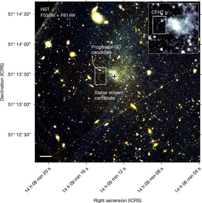
Images of UGC 9050-Dw1 were obtained with the Hubble Space Telescope (HST) Advanced Camera for Surveys (ACS), using the Wide Field Channel (WFC) and the F555W and F814W filters. The images have an angular resolution of 0.1″ and exposure times of 2,406 s and 2,439 s, respectively. Observations were completed in September 2022 under HST programme ID 16890 (ref. ⁵²). The resulting UGC 9050-Dw1 images were presented in ref. ¹⁷, processed with the standard HST CALACS calibration pipeline and made available through the STScI/MAST archive.

The Canada–France–Hawaii Telescope (CFHT) observed the same sky region with MegaCam in 2005 as part of the CFHT Legacy Survey. UGC 9050-Dw1 was first identified during a semi-automated search for diffuse dwarf galaxies¹⁹. The target lies within both the W3-1-3 and W3-2-3 survey fields, which cover the u, g, r, i and z bands and provide ten CFHT images in total. Because of their signal-to-noise ratios, the stream-like feature cannot be identified confidently in the u- or z-band data. Exposure times, limiting depths and seeing measurements for the CFHT observations are reported in ref. ⁵³. The calibrated CFHT images were processed with the MegaPipe pipeline and are available from the Canadian Astronomy Data Centre.

For visualization, we smoothed the HST and CFHT images with Gaussian kernels having σ values of 3 and 1.5 pixels, respectively. The region surrounding UGC 9050-Dw1 is displayed in every available filter in Extended Data Fig. 1. All quantitative measurements and analyses use the original, unsmoothed images.

Data analysis

We initially identified the candidate stellar stream by visual inspection. We then applied the rolling Hough transform⁵⁴ across a range of hyperparameters. In every case, the algorithm recovered both the position and curvature of the stream candidate, supporting the original visual detection.

As shown in the left panels of Extended Data Fig. 2, we rotate the images into a coordinate system aligned with the stream. In this frame, (ϕ₁, ϕ₂) denotes stream longitude and latitude^55,56. We trace the stream using a polynomial fitted to manually selected points in the F814W image. Around this track, we construct a curved mask with constant width while excluding the globular cluster (GC) candidate. Equivalent masks are placed on either side of the stream to measure the background. We estimate the stream width by sampling slices perpendicular to the curved track at pixel-sized intervals. The sampled pixels are averaged along the track to produce the mean brightness of the stream candidate and its surrounding regions.

The right panels of Extended Data Fig. 2 show the resulting perpendicular surface-brightness profiles, calculated parallel to the curved stream track. We divide the stream into six segments to test whether any individual contaminating object dominates the measurement. For each segment and for the full stream, we fit a Gaussian profile with a linear background offset. Because the sampling method oversamples the inner portion of the curve relative to the outer portion, the inner region would otherwise have a smaller formal uncertainty and disproportionately influence the fit. We therefore adopt the mean of all standard deviations as a uniform error.

The Gaussian standard deviation provides an estimate of the stream width and its associated parameter uncertainty. Since σ measures the deviation from the mean, μ, the full width from μ − σ to μ + σ is 2σ. We refer to this measurement as w_±σ. The width enclosing approximately 95% of the Gaussian area, extending to 2σ on either side of the mean, is denoted by w_±2σ. To recover the intrinsic physical width, we subtract the instrumental point spread function (PSF) in quadrature. For the HST data, we use a full width at half maximum of 0.1″.

The CFHT seeing, 0.88″, is comparable to the measured feature width in the CFHT images, where w_±σ = 1.1″. We therefore use the higher-resolution HST width for the remainder of the analysis.

A relatively bright object near the track at approximately ϕ₁ = −4 increases the measured stream width. Restricting the analysis to the track before this object produces w_±σ = 52 pc. Conversely, the low surface brightness of the stream may mean that we detect only its brightest central region, potentially underestimating the true width. Extended Data Fig. 6 shows that simulated GC streams inserted into the images have similar apparent widths.

We quantify the prominence of the stream candidate by summing the counts within the on-stream mask and the off-stream background masks. After subtracting the mean background flux from the stream signal, we compare the residual with the background standard deviation using \(({f}_{{\rm{stream}}}-\,{\overline{f}}_{{\rm{background}}})/{\sigma }_{{\rm{background}}}\).

The Gaussian model used for the width measurement also provides a signal-to-noise estimate. We calculate this by comparing the fitted amplitude with its uncertainty, \(A/\sqrt{{\sigma }_{A}}\). This uncertainty includes errors in the mean brightness values used in the fit. Neither prominence estimate includes flux from the GC candidate; both measurements are based exclusively on light from the stream candidate.

The overall statistical significance has three separate components: the probability that the feature is a stream, the probability that such a stream would be detected, and the statistical significance of the measured signal if the first two conditions are satisfied. The significance quoted here refers only to the final component—the statistical strength of the signal in the data.

To compare the stream and cluster colours with other GC candidates in the host ultra-diffuse galaxy (UDG), we sum their fluxes in the two available HST filters. We define the stream region as a curved, constant-width mask around a polynomial fitted to manually selected points along the track. The adopted width is w_±2σ = 16.8 pixels = 143.7 pc. The GC candidate is measured within a circular mask 20 pixels, or 170.6 pc, wide. Its aperture radius is selected using a photometric growth-curve analysis similar to that described in ref. ⁵⁷, ensuring that most of the source flux is included. The stream and progenitor masks are kept separate. Their locations are shown with blue and purple outlines, respectively, in Extended Data Fig. 3. Magnitudes are reported in the Vega system and corrected for Galactic extinction using the values from ref. ⁵⁸, calculated with the NASA/IPAC Extragalactic Database (NED) extinction calculator.

Reliable colour measurements require subtraction of the background in a nearby region with approximately equal area (see, for example, ref. ⁵⁹). The complex morphology of UGC 9050-Dw1 makes the ideal background region difficult to define, and the measured colour can vary substantially depending on the selected area. We therefore average measurements from several regions distributed on both sides of the stream candidate, as illustrated in Extended Data Fig. 3. Colour uncertainties include the variation among the individual background regions and the uncertainty in the flux measured in each filter, estimated from the standard deviation of the pixel values.

The ACS pixel scale is 0.05″ per pixel, corresponding to 8.53 pc at the distance of UGC 9050-Dw1. This scale is comparable to the expected size of globular clusters, which are typically a few parsecs across⁶⁰. For this reason, ref. ¹⁷ treats the GC candidates as point sources. A partially disrupted cluster, however, should have a larger physical extent, while a stellar stream is inherently non-point-like. We therefore analyse both objects as extended sources, using the regions shown in Extended Data Fig. 3. The GC candidate was not included in the final GC sample of ref. ¹⁷. Its selection criteria indicate that it was excluded because of its roundness, sharpness and/or magnitude uncertainty. A tidally disrupting GC is expected to be more elongated and diffuse than an intact cluster, naturally explaining its failure to meet all three criteria.

We integrate the flux within the stream mask shown in Extended Data Fig. 3 to determine its surface brightness. After background subtraction, we obtain 27.0 ± 0.1 and 26.1 ± 0.1 mag arcsec⁻² in the HST F555W and F814W filters, respectively.

To investigate the stellar populations that could produce the observed stream, we generate a grid of isochrones spanning different ages and metallicities. Stars are sampled from a simple initial mass function (IMF), following \(\frac{{\rm{d}}N}{{\rm{d}}m}\propto {m}^{-0.5}\) (ref. ⁶¹), and truncated according to the range of stellar masses that survive in each isochrone. We obtain stellar magnitudes by interpolating isochrone tracks generated for the HST and CFHT filters through the colour–magnitude diagram input form⁶², using the PARSEC version 1.2S evolutionary model⁶³.

We distribute the simulated stars across the observed stream area, including the presumed hidden arm, and calculate the resulting surface brightness. We then reduce the population until only one isochrone produces a surface brightness consistent with the HST observations. This population is detectable only through the brightest isochrone in our model grid. Its total mass therefore provides a lower limit for a stream covering the observed area and producing the measured brightness.

We find that a progenitor with an initial stellar mass as low as M_⋆,tot = 1.65 × 10⁵ M_⊙ can reproduce the present-day stream surface brightness if it contains an 8-Gyr-old stellar population with [M/H] = −1.0.

The detailed mass-loss history of the GC candidate is unknown. To estimate the combined mass of the stream and progenitor, we assume that the stream-to-cluster brightness ratio is a suitable proxy for their mass ratio. If the two stream arms are identical, this gives M_stream/M_total ≈ 0.75. We use this ratio to scale the inferred stream mass and estimate the total progenitor mass.

For the Pal 5-like stream model, we estimate the degree of disruption using the method described in ref. ³⁷. We adopt an isochrone with an age of 11.3 Gyr and metallicity [M/H] = − 1.3. Pal 5 contains approximately 3,000 stars in the DECam g band between magnitudes 23 and 20 (ref. ⁵⁹). We therefore sample the IMF until this number is reached and calculate the resulting population surface brightness. We repeat the procedure for samples containing 5, 10 and 20 times this number of stars, corresponding to the same multiples of the Pal 5 mass. The 20× sample produces a surface brightness consistent with the HST measurements. This calculation assumes that the stream has experienced mass loss comparable to that of Pal 5.

Generative stream models

We generate model stellar streams with the X-Stream sampler⁶, which uses the particle-spray method⁶⁴ implemented in the GPU-based streamsculptor code⁶⁵. Escape conditions are fixed according to ref. ⁶⁴. These particle-spray simulations are calibrated to reproduce more computationally demanding N-body models of GC dissolution. Consequently, our results depend on the adopted escape conditions.

We model the streams within a dark-matter halo potential designed to represent the diffuse dwarf galaxy, characterized by inner and outer slopes, γ and β, respectively; see equation (1) in ref. ⁶. Baryonic matter is excluded because it contributes only a small fraction of the total mass compared with the estimated system mass, M_* ≈ 10⁷ M_⊙ within the half-light radius¹⁷. The dark-matter halo is therefore treated as a representation of the entire diffuse dwarf system.

We define the model coordinate system by transforming the candidate GC progenitor and the centre of UGC 9050-Dw1 from right ascension and declination into a galactocentric rest frame. Using astropy⁵⁶ and a distance of 35.2 Mpc, we place UGC 9050-Dw1 at the origin. The x and z axes lie in the plane of the sky, while the y axis follows the line of sight towards the observer. The progenitor’s projected position, (x, z), is fixed in all models.

Within this coordinate system, we define a mask for the observed stream extending to the left of the candidate GC progenitor. To evaluate the impact of the adopted stream width, we use two masks. The fiducial mask has a width of w_±2σ = 143.7 pc, while the second has a width of 185 pc, corresponding to w_±3σ. A grid of control points within each mask represents the observed stream and serves as input for the X-Stream sampler. We generate control points only on the left side because no right-hand extension is confidently detected.

We convert the control points into a kernel density estimate (KDE). For every model stream, X-Stream generates a KDE and uses a Kullback–Leibler divergence test^66,67 to compare it with the KDE derived from the control points; methodological details are provided in ref. ⁶. The preferred models minimize this divergence. Particle-spray models do not reproduce the detailed density variations along the stream. Instead, X-Stream uses control points and inverse-density weighting to smooth over small-scale features. Models wider than the data contain excess density relative to the control points and are therefore disfavoured.

We draw a bounding box around the stream mask so that models are not penalized for extending beyond the mask or to the right of the progenitor. However, models that do not reach the full observed stream length are penalized.

To explore which orbital configurations, progenitor properties and halo parameters reproduce the observed stream, we vary ten free parameters with uniform, flat priors. Only the progenitor’s projected position is fixed, as listed in Extended Data Table 1. We test dark-matter halo concentrations of c = 2 and c = 5, motivated by refs. ^3,5. X-Stream uses nested sampling to explore the large parameter space and returns the likelihood for each model, together with the likelihood surface and 68% and 95% credible regions for all parameters.

Stellar streams have known degeneracies in their orbital direction across the plane of the sky; see Figs. 10 and 8 in refs. ^6,33, respectively. We therefore sample only half of the unit sphere in velocity space. This creates equivalent solution islands in which the model stream travels in the opposite direction, exchanging the leading and trailing arms. These solutions provide equally good fits, while their distance gradients remain unchanged; see Figs. 10 and 9 in refs. ^6,33, respectively. All free and fixed X-Stream parameters are listed in Extended Data Table 1, and detailed parameter definitions are given in ref. ⁶.

To determine which portions of the model streams could be detected in the HST observations, we create mock observations of three stellar-stream scenarios:

1. 1)

   Lower-bound stream: a stream with a progenitor mass of 1.65 × 10⁵ M_⊙, metallicity [M/H] = −1.0 and age 8 Gyr. These properties are motivated by the surface-brightness analysis, which indicates that such a stream should be detectable in the HST data. We populate the model with 2.8 × 10⁵ stars, matching the simulated population with a mass of 1.65 × 10⁵ M_⊙.

2. 2)

   20× Pal 5-like stream: a stream with a progenitor mass of 2 × 10⁶ M_⊙, metallicity [M/H] = −1.3 and age 11.3 Gyr. Our surface-brightness analysis predicts that this stream should also be visible in the HST images. We populate it with 1.17 × 10⁶ stars, based on the corresponding simulated stellar population.

3. 3)

   Dwarf-like stream: a stream with a progenitor mass of 2 × 10⁷ M_⊙, designed to represent a more massive dwarf-galaxy stream. We use the same stellar population as in the 20× Pal 5-like model for direct comparison and to represent the additional mass as dark matter.

For every model, we sample the IMF up to the stellar mass that survives to the present day. Each star is assigned an F555W and F814W magnitude by interpolating the selected isochrone. We distribute the stellar flux across the model stream, add Poisson noise and inject the resulting mock stream into HST images in both filters. The injected flux is convolved with an empirical PSF described in ref. ⁶⁸, using PSF models from ref. ⁶⁹. For visual comparison, each stream is inserted into an approximately empty region near the Oyashio stream.

When estimating the expected surface brightness, we assume that every simulated star lies inside the stream mask. This assumption is inaccurate, particularly for the broader dwarf-like stream. To make that model visible, we increase its brightness by a factor of 5. This demonstrates that a stream covering a larger area requires a more massive stellar component to produce the same surface brightness. The mock images are stacked using the procedure shown in Fig. 1 and presented in Extended Data Fig. 6.

This analysis depends on several assumptions, including the selected isochrones, the degree of tidal disruption and the adopted stream-modelling prescriptions. Nevertheless, the mock observations provide a zeroth-order assessment of which regions of each model stream may be detectable in the HST data.