Infrared Absorption Spectroscopy of a Single Polyatomic Molecular Ion

Molecule generation

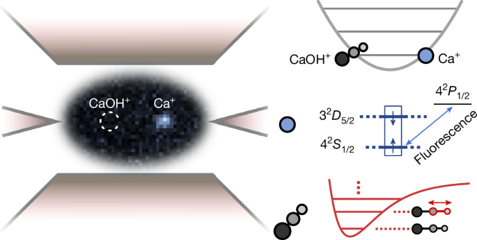
Our experiment uses a mixed-species two-ion crystal containing ⁴⁰Ca⁺ and ⁴⁰CaOH⁺ confined in a linear Paul trap²⁸. To generate the calcium hydroxide molecular ion, we first load two ⁴⁰Ca⁺ ions into the trap and then introduce water vapour through a leak valve connected to a gas chamber. The chamber contains predominantly water vapour at a pressure of approximately 10⁻⁶ mbar.

During molecule formation, a 397 nm laser drives the 4²S_1/2 → 4²P_1/2 dipole transition in ⁴⁰Ca⁺. This laser Doppler-cools the ion crystal while a camera monitors calcium-ion fluorescence. Because CaOH⁺ does not fluoresce at this wavelength, the formation of a molecular ion causes one ion to appear dark on the camera. Once this dark ion is detected, we close the leak valve and perform mass spectrometry by measuring the motional frequency of the ion crystal²⁴. This confirms the formation of CaOH⁺. Molecule generation typically takes approximately 5 min. After the valve is closed, the vacuum pressure returns to about 10⁻¹⁰ mbar within a few minutes.

Following the formation of the mixed-species ion crystal, collisions with residual background gas can cause the atomic and molecular ions to exchange positions over several seconds. For cat-state spectroscopy, we use only one of the two possible ion configurations because each configuration has a different motional frequency. This difference is likely caused by imperfect micromotion compensation²⁴.

Before each spectroscopy sequence, we identify the ion-crystal configuration during Doppler cooling. If the ions are in the undesired configuration, we attempt to switch their positions randomly by displacing the crystal radially from its trapping position. This process is repeated until the ions return to the required configuration.

Cat-state engineering

To measure photon recoil, we prepare a non-classical motional state using a bichromatic laser beam directed at the ⁴⁰Ca⁺ ion. The two frequency components have equal intensity and are detuned by −ω_z and +ω_z from the atomic quadrupole transition between |↑⟩ and |↓⟩. Here, ω_z denotes the in-phase motional frequency of the ion crystal⁴. The Lamb–Dicke parameter for this quadrupole transition is

where M_a is the atomic mass, \({k}_{z,{\rm{a}}}\) is the component of the quadrupole-transition laser wavevector along the trap axis, and \({e}_{z,{\rm{a}}}\) is the atomic-ion participation factor for the in-phase motional mode. In the Lamb–Dicke regime, the light–ion interaction Hamiltonian is³⁸

Here, Ω₀ is the Rabi frequency, \({\hat{a}}^{\dagger }\) and \(\hat{a}\) are the creation and annihilation operators for the harmonic oscillator describing in-phase motion, and ϕ_r and ϕ_b are the phases of the red- and blue-detuned frequency components, respectively. The term h.c. denotes the Hermitian conjugate.

This interaction produces a spin-dependent displacement described by ϕ_± = (ϕ_b ± ϕ_r)/2:

For ϕ₊ = 0, the Hamiltonian becomes

As a result, the two \({\hat{\sigma }}_{x}\) eigenstates |±⟩ undergo opposite motional displacements, \(\widehat{D}(\alpha )\) and \(\widehat{D}(-\alpha )\). For a pulse duration T, the displacement amplitude is \(\alpha =-{\rm{i}}{\eta }_{{\rm{a}}}{\varOmega }_{0}T{{\rm{e}}}^{{\rm{i}}{\phi }_{-}}/2\).

The resulting cat state is a superposition of two motional wave packets correlated with different atomic states, as shown in equation (2). Applying the same interaction with ϕ₊ = π for the same duration reverses the spin-dependent displacement and recombines the wave packets. Photon absorption is timed to occur between cat-state generation and reversal. The resulting momentum recoil produces a geometric phase difference between the two wave packets, which is detected by measuring the final atomic state, as described in equation (3).

Experimental imperfections

We describe experimental imperfections with a physically motivated model that includes atomic and motional decoherence. In this experiment, these effects primarily arise from magnetic-field fluctuations and trap-voltage fluctuations, respectively. We simulate cat-state photon-absorption detection using Lindblad master equations with the following collapse operators:

Here, T_spin is the coherence time of the atomic two-level system, while T_motion is the coherence time of a superposition between the motional ground state and first excited state. Ramsey measurements performed on the experimental timescale give T_spin = 2.8(3) ms and \({T}_{\mathrm{motion}}=8{5}_{-35}^{+98}\,\mathrm{ms}\). The motional coherence time is substantially longer than the cat-state spectroscopy sequence, resulting in the relatively large uncertainty in its estimated value.

Using these coherence times, we calculate the expected experimental signal for different cat-state amplitudes and photon-recoil kick sizes, as shown in Fig. 3. The purple-shaded area represents simulations incorporating one standard deviation of the atomic and motional coherence times. The primary effect of these imperfections is a reduction in signal amplitude. We also describe this loss with the heuristic model in equation (5), which multiplies the ideal contrast in equation (4) by a factor \({{\mathcal{S}}}_{\max }\). For a cat-state amplitude of |α| = 6.5(7), fitting equation (5) to measurements at different kick sizes gives \({{\mathcal{S}}}_{\max }\) = 0.52(3).

The parameter \({{\mathcal{S}}}_{\max }\) captures decoherence and changes with the cat-state amplitude and measurement-sequence duration. In measurements of effective photon-absorption probability versus the number of femtosecond laser pulses, n_pulse, shown in Fig. 4a, changing the pulse number also changes the interval between cat-state generation and reversal. Consequently, \({{\mathcal{S}}}_{\max }\) varies with n_pulse. We characterize this effect using electric-kick measurements and model it as

for |α| = 6.5(7), where τ_d = 0.92(6) ms. The measured signals are adjusted accordingly for different numbers of laser pulses.

Timing jitter in photon absorption relative to the ion-crystal motion is another possible source of error. The recoil-induced geometric phase difference, Φ = 2η_mRe(α), depends on the phase relationship between the cat state and the photon-recoil displacement. This relationship is determined by the free-evolution time between cat-state generation and photon absorption, T_wait.

In our experiment, photon absorption is synchronized with femtosecond laser pulses. We trigger cat-state generation from the periodic laser pulses, achieving timing jitter below 10 ns. Because this is much shorter than the ion oscillation period, the free-evolution time T_wait remains effectively constant. The trap frequency ω_z and laser repetition rate f_rep also affect the phase. We set the trap frequency to an integer multiple of the repetition rate, ω_z/2π = 4 ⋅ f_rep, so that photon recoil from each femtosecond pulse produces the same Re(α). Variations in the trap frequency or repetition rate would otherwise change the phase of the signal from pulse to pulse.

The measured variation in ω_z/2π is approximately 50 Hz, while fluctuations in f_rep are below 10 Hz. The resulting variation in arg(α) is less than 3.2 × 10⁻² over the maximum T_wait and can therefore be neglected.

Quantum-chemical calculations

We calculate the vibrational transition frequencies and intensities of CaOH⁺ ab initio using advanced quantum-chemical methods. The analysis focuses on the observed O–H stretching mode, which produces the strongest spectral band.

First, we calculate an accurate potential energy surface using coupled-cluster electronic-structure methods. This surface provides the harmonic frequencies and normal coordinates for the molecular stretching modes. The best estimate of the O–H harmonic frequency is 3,950 cm⁻¹. We then neglect coupling between different normal modes, reducing the multidimensional anharmonic vibrational problem to independent one-dimensional problems along the normal coordinates.

The one-dimensional Schrödinger equation for nuclear motion along the O–H-dominated normal coordinate is solved using the discrete variable representation method³⁹. The resulting vibrational energies and wavefunctions give a fundamental transition frequency of 3,792 cm⁻¹ and an oscillator strength of 3.7 × 10⁻⁵. Finally, we restore coupling between the fundamental O–H stretch, Ca–O stretch and Ca–O–H bending modes using vibrational second-order perturbation theory (VPT2)⁴⁰. This lowers the O–H fundamental frequency by 9.5 cm⁻¹, giving a final predicted value of 3,783 cm⁻¹.

The electronic-structure calculations use correlation-consistent, polarized, weighted core–valence basis sets augmented with diffuse functions, aug-cc-pwCVnZ-PP, where n = T, Q and 5 (refs. ^41,42,43). The ten core electrons of calcium are represented by the ECP10MDF effective core potential, which accounts for relativistic effects⁴⁴.

The potential energy surface is generated with a composite scheme in which the total energy is written as the sum of three components: (1) the Hartree–Fock mean-field energy; (2) the primary correlation contribution calculated using coupled-cluster theory with single, double and noniterative triple excitations, CCSD(T)⁴⁵; and (3) the contribution from triple excitations omitted by CCSD(T) but included in CCSDT⁴⁶. The final contribution is calculated with a triple-ζ basis set, while the first two contributions are extrapolated to the complete-basis-set limit using basis sets through quintuple-ζ. Three-point exponential⁴⁷ and two-point 1/n³ extrapolation formulas are used for the Hartree–Fock and correlation energies, respectively.

The permanent electric dipole moment is calculated analytically at the CCSD(T)/aug-cc-pwCV5Z level. Its value for the ground vibrational state is 6.2 D.

For linear CaOH⁺, the potential energy surface is calculated as a function of the Ca–O and O–H bond lengths on a uniform two-dimensional grid with 0.002 bohr spacing around the equilibrium geometry²⁸. The surface is interpolated using a natural cubic spline. After determining the normal coordinate, we calculate 33 electronic energies along that coordinate. The VPT2 correction is estimated from anharmonic constants obtained at the CCSD(T)/aug-cc-pwCVTZ level.

All electronic-structure and VPT2 calculations are performed using CFOUR v.2.1⁴⁹.

Molecular excitation dynamics

We model the O–H stretching excitation dynamics of CaOH⁺ as a two-level system consisting of the vibrational ground state |g⟩ and first excited state |e⟩. The molecular laser pulses are assumed to have Gaussian temporal intensity profiles with an FWHM duration of \(\tau =2{\tau }_{\sigma }\sqrt{2\mathrm{ln}2}\), where τ_σ is the one-standard-deviation pulse duration.

The molecule therefore experiences the following time-dependent electric field:

Here, ω and ϕ are the laser centre frequency and phase, respectively, while E₀ is the peak electric-field amplitude and c.c. denotes the complex conjugate. The peak electric field is determined from the average laser intensity, I_avg, according to \({E}_{0}=\sqrt{{I}_{\mathrm{avg}}/({f}_{\mathrm{rep}}\tau \sqrt{{\rm{\pi }}/\mathrm{ln}2}\cdot {\epsilon }_{0}c)}\).

The light–molecule interaction is described by

where the transition dipole moment μ_eg is related to the oscillator strength through \({\mu }_{eg}=\sqrt{{f}_{eg}\cdot 3\hbar {e}^{2}/{m}_{e}{\omega }_{0}}\). The angle θ represents the angle between the molecular axis and the laser-polarization direction.

In the interaction picture and under the rotating-wave approximation, the Hamiltonian becomes

where Δ = ω − ω₀ is the detuning from the transition frequency ω₀, and Ω(t) is the time-dependent Rabi rate:

We use this model to reproduce the experimental results without free parameters through Monte Carlo simulations of the light–molecule interaction in equation (15). For every laser pulse in each simulation trial, we randomly select the optical phase ϕ, which is not stabilized between pulses, and the molecular orientation angle θ. This assumes that the molecules are randomly oriented in the experiment.

The single-pulse Rabi rate is calculated from the ab initio transition frequency and oscillator strength described in the “Quantum-chemical calculations” section, together with the experimentally measured laser parameters.

Femtosecond pulses are generated by an ORPHEUS-HP optical parametric amplifier pumped by a CARBIDE-CB5 femtosecond laser, both manufactured by Light Conversion. The light delivered to the ions is linearly polarized in the vertical plane. Given our magnetic-field geometry, this polarization produces an equal superposition of σ₊ and σ₋ components.

The average intensity at the ion position is 1.1(1) × 10⁴ W cm⁻². We measure the laser spectrum with a Redstone OSA305 optical spectrum analyser to determine the centre wavelength and linewidth at each frequency used in the absorption spectrum. Although absorption lines from water vapour are visible along the beam path, we assume they do not influence the molecular absorption measurement because of power broadening.

The measurement shown in Fig. 4 uses a laser centre frequency of ν = 3,703.3(2) cm⁻¹ and an FWHM linewidth of 126.7(4) cm⁻¹. The simulation uses these values and assumes Fourier-transform-limited pulses with an FWHM duration of 116.2(4) fs. For the absorption spectrum in Fig. 4d, experimental data are compared with simulations using the Fourier-transform-limited pulse duration determined from the measured centre frequency and linewidth at each optical parametric amplifier wavelength setting.

Non-destructive state detection

Photon-absorption detection can enable effective, non-destructive measurement of selected molecular states. Here, we outline a scheme that acts on the two lowest vibrational states of a molecular mode. Consider the three lowest vibrational states, |0⟩, |1⟩ and |2⟩. We assume that selective laser operations can address these states spectroscopically because molecular anharmonicity gives each transition a distinct frequency.

The proposed method performs a projective measurement in the {|0⟩, |1⟩} subspace. Assume that the molecule is prepared in a superposition of vibrational states while the shared ion motion and atomic ion are both in their ground states:

We first generate an atom–motion cat state, producing

We then configure the cat-state spectroscopy sequence so that photon absorption completely flips the atomic electronic state when Re(α) = π/(4η_m). The combined molecular, atomic and motional state is

Next, a laser pulse transfers the population from |1⟩ to |2⟩ while applying a displacement operator to the shared ion motion:

After reversing the cat-state-generation sequence, the system evolves to

This state entangles the molecular vibrational degree of freedom with the atomic electronic state. Measuring the atomic state therefore projects the molecule into either |0⟩ or |2⟩. If the molecule is projected into |2⟩, its population can be transferred back to |1⟩. The complete sequence provides a non-destructive method for detecting selected molecular vibrational states.