


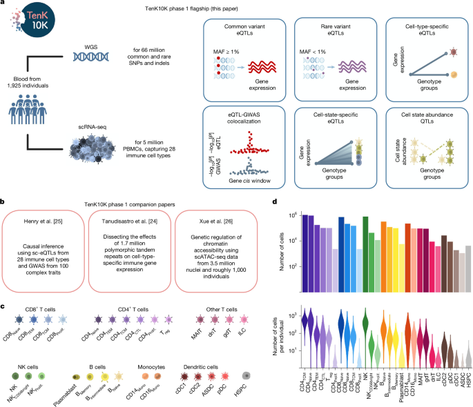
Researchers analyzed whole-genome sequencing (WGS) and single-cell RNA sequencing (scRNA-seq) data from Australian biomedical research cohorts to investigate genetic effects on gene expression across 28 immune-cell types. Blood samples were collected from 2,339 consenting participants in the Tasmanian Ophthalmic Biobank (TOB) and the BioHEART study. After donor, variant and cell-quality control, including restriction to participants of European ancestry, the final dataset included 1,925 individuals and 5,438,679 cells. The study used common- and rare-variant association tests, chromatin-accessibility and functional annotations, fine mapping, colocalization with disease and blood-trait GWAS data, and analyses of cell states and cell abundance.
Cohorts and participants
Blood samples came from two Australian biomedical research cohorts: the Tasmanian Ophthalmic Biobank (TOB), covered by ethics protocol 2020/ETH02479, and the BioHEART study, covered by ethics protocol 2019/ETH08376.
The TOB cohort comprised 983 people—562 female and 421 male—recruited between January and February 2018 by the Royal Hobart Hospital and the Menzies Institute of Medical Research in Tasmania, Australia. Participants were at least 18 years old, had no signs of ocular disease and self-reported British, Scottish or Irish ancestry.
The BioHEART63 cohort comprised 1,356 people—561 female and 795 male—recruited between 29 March 2016 and 2 May 2023. Participants attended study sites for clinically indicated cardiovascular imaging or presented acutely with ST-elevation myocardial infarction. Eligibility required participants to be at least 18 years old and to have a cardiac disorder, or be undergoing investigation for a suspected cardiac disorder. Relevant conditions and procedures included acute myocardial infarction, suspected coronary artery disease, cardiothoracic or vascular surgery, and plastic surgery involving resection of vascularized tissue.
After donor, variant and cell-quality control, and selection of individuals of European ancestry, 1,925 participants remained: 950 from TOB and 975 from BioHEART.
Ethics and sample processing
The study complied with relevant ethical regulations and was overseen by Human Research Ethics Committees at the Royal Children’s Hospital in Melbourne, Northern Sydney Local Health District, St. Vincent’s Hospital in Sydney and the University of Tasmania in Hobart. All participants provided informed consent.
For the TOB16 cohort, blood was collected into one 8-ml heparin cell-preparation tube and one 9-ml EDTA tube per participant. BioHEART aliquots were stored at −80 °C.
DNA from BioHEART buffy-coat samples was extracted by the Australian Genome Research Facility using the QIAamp96 DNA QIAcube HT kit. TOB DNA was extracted at the Menzies Institute of Medical Research at the University of Tasmania using the QIAamp Blood Mini Kit. For some TOB samples that failed initial sequencing quality-control checks, DNA was extracted again from peripheral blood mononuclear cells using the Qiagen DNeasy Blood and Tissue Kit. The samples were eluted in AE buffer by the Garvan Molecular Genetics laboratory service.
DNA concentrations were measured for all samples by fluorometric quantitation with Promega’s Quantifluor before sequencing.
Whole-genome sequencing
WGS data were generated for all 983 TOB participants and all 1,356 BioHEART participants. Libraries were prepared with the KAPA PCR-free v.2.1 kit from Roche for TOB samples and the Illumina DNA PCR-free kit for BioHEART samples. Short-read sequencing used Illumina 2 × 150-base-pair chemistry on a NovaSeq 6000 instrument, targeting a mean coverage of 30×. Library preparation and sequencing were performed by the Garvan Sequencing Platform.
Read alignment and variant calling
Read alignment and variant calling followed GATK-DRAGEN Best Practices. BioHEART reads were aligned from FASTQ files, while TOB reads were aligned from CRAM files, against the masked GRCh38 reference genome available in the GATK resource bundle. The analysis used a fork of DRAGMAP v.1.3.1. For CRAM-based alignment, bazam was first used to convert reads back to FASTQ format.
Single-nucleotide polymorphisms and indels were called with GATK4 HaplotypeCaller in DRAGEN mode. The resulting genomic VCF files were combined with Hail’s VDS Combiner and stored in variant dataset (VDS) format.
Sample quality control and ancestry
Individuals were removed for contamination of at least 5% (FREEMIX ≥ 5%), a chimera rate of at least 6.3% (PCT_CHIMERAS ≥ 6.3%), a median insert size below 250 bp, sex aneuploidy, or disagreement between reported and observed sex. Samples were also inspected for outlying numbers of singleton variants, heterozygous-to-homozygous variant ratios, transition-to-transversion ratios and insertion-to-deletion ratios. Ancestry outliers were not excluded on the basis of these metrics alone.
The researchers extracted high-quality sites consisting of an LD-pruned set of autosomal, biallelic variants with allele frequency above 0.01, call rate above 99% and InbreedingCoeff above −0.25 from the 1,000 Genomes Project and the Human Genome Diversity Project. Samples with a call rate below 0.85 across these sites were removed.
Related individuals were identified using Hail’s PC-Relate implementation and confirmed with somalier relate v.0.2.15. In groups containing second-degree or closer relatives, defined by a kinship coefficient above 0.088, the sample with the highest-quality scRNA-seq data was retained, based on cell numbers and cell-type composition. If single-cell data quality was equivalent, the sample with the greatest mean sequencing depth on chromosome 20 was retained.
Ancestry was inferred in the high-quality, unrelated samples after combining them with reference samples from the 1,000 Genomes Project and the Human Genome Diversity Project. Principal components were calculated with gnomAD’s run_pca_with_relateds method using the same high-quality sites used for call-rate assessment. Ancestry labels were assigned according to genetic similarity to reference samples of known ancestry. Only participants assigned to the European cluster were retained for association testing.
Variant quality control
Allele-specific Variant Quality Score Recalibration (AS-VQSR) was performed with GATK v.4.2.6.1 on all quality-control-pass, unrelated samples, regardless of ancestry. Default training resources and priors were used. For SNPs, these were hapmap (15), omni (12), 1,000 Genomes (10) and dbSNP (7). For indels, they were mills (12), axiomPoly (10) and dbSNP (2).
The features used for SNPs and indels were AS_ReadPosRankSum, AS_MQRankSum, AS_QD, AS_FS and AS_SOR; AS_MQ was also used for SNPs. Sites failing the AS-VQSR site-level filter were removed.
Within the European-only association dataset, variants were removed if they had no high-quality genotype calls or showed an excess of heterozygotes relative to Hardy–Weinberg expectations. A high-quality genotype was defined as genotype quality (GQ) ≥ 20, sequencing depth (DP) ≥ 10 and allele balance above 0.2 for heterozygotes. Sites with more than 15% missingness were also removed.
Single-cell RNA sequencing
scRNA-seq data were generated from peripheral blood mononuclear cells from 1,036 TOB participants in OneK1K16 and 1,012 BioHEART63 participants. The experimental workflow and key processing steps are shown in Supplementary Fig. 40.
Pooling and sequencing
TOB samples had previously been pooled during preparation of the OneK1K project, with each pool containing 1,214 individuals16. To increase the number of cells captured per participant, two pools of 24–28 individuals were combined at a time, weighted by cell viability, and loaded across three sequencing lanes. Each lane targeted 40,000 cells, or 120,000 cells in total, corresponding to a target of up to 5,000 cells per participant. “Maxi pools” containing four combined pools, or 96–112 individuals, were also sequenced across two separate lanes to compensate for potentially low cell numbers.
BioHEART samples were pooled specifically for this project, with eight participants per pool and one sequencing lane per pool. The target was 40,000 cells per pool, or approximately 5,000 cells per participant. Pools with low cell viability were sometimes sequenced again to increase cell recovery.
Cells were captured with the 10x Genomics single-cell 3′ gene-expression high-throughput kit v.3.1 on a Chromium X instrument. TOB cells were recaptured from biobanked OneK1K material using the updated 10x chemistry and high-throughput kit. Long-term cryopreservation resulted in a smaller proportion of monocytes in TOB than in BioHEART, as described in Supplementary Note 1. Libraries were prepared and sequenced on an Illumina NovaSeq 6000.
Alignment, donor assignment and cell typing
Reads were aligned to the GRCh38 reference with Gencode release 44 and Ensembl 110 using STAR64 within 10x Genomics Cell Ranger v.7.2.0. Cell Ranger also estimated the number of captured cells. CellBender65 v.0.3.0 produced substantially different cell estimates, so those results were discarded.
Donors were assigned and doublets—droplets containing more than one cell—were identified with Demuxafy66 v.2.1.0. Vireo67 was used to assign cells to donors within each sequencing library. TOB analyses used SNP-array genotypes from the OneK1K data, while BioHEART analyses used common biallelic WGS SNPs with minor allele frequency above 5%. A small number of participants lacked genotype data; Vireo can incorporate the expected number of participants in a pool with or without genotypes.
Demuxafy was also used to run scds68 and ScDblFinder69. Majority voting across Vireo, scds and scDblFinder determined the final doublet calls for each sequencing library.
Cells were assigned to immune-cell types using a combined approach recommended by the single-cell eQTLGen consortium28. The approach used scPred70, hierarchical progressive learning with scHPL71, and Azimuth as the reference dataset72, following the documentation at the WG2 pipeline classification site. Scanpy objects were converted to Seurat73 objects for this step.
CellTypist74,75 v.1.6.2, using the “Immune_All_High” model, was used as an independent check and showed good concordance. The combined method provided greater resolution, identifying 28 cell types compared with 18 from CellTypist, so the 28-cell-type classification was used for subsequent analyses.
Cell-level quality control
Quality control was performed with Scanpy v.1.8.2. Within each library, cells were removed if more than 20% of their reads were mitochondrial, fewer than 800 reads were detected, or fewer than 1,000 or more than 10,000 genes were detected. Individuals with abnormal cell-type composition or fewer than 100 cells were also excluded.
After cell and sample quality control using both scRNA-seq and WGS data, 5,438,679 cells from 1,925 individuals remained for analysis.
Common- and rare-variant eQTL mapping
The researchers used SAIGE-QTL27 to test common- and rare-variant associations with single-cell gene expression. The method uses a Poisson mixed model to represent single-cell counts and repeated observations from the same individual, with computational procedures designed to improve speed, scalability and storage efficiency. Both single-variant and set-based tests were performed.
eQTLs were mapped independently in each of the 28 cell types. Calibration was assessed by shuffling participant identifiers and repeating the analysis for the most abundant cell type, CD4TCM cells. These tests showed no evidence of false-positive inflation for either common- or rare-variant analyses.
Model specification
For every gene and cell type, a single null model was fitted for both common- and rare-variant testing. The Poisson model used raw single-cell expression counts as the outcome and included sex, age, seven genotype principal components, five cell-type-specific expression principal components, cohort status, the percentage of counts from mitochondrial genes and total counts as covariates.
Only genes expressed in at least 1% of cells in a cell type were tested. The model failed to converge for 0.27% of gene–cell-type combinations, which were excluded.
Common variants
Common-variant effects were tested with the SAIGE-QTL single-variant test. The analysis included SNPs and indels with minor allele frequency (MAF) ≥ 1% and less than 15% missingness, considering only cis effects within ±100 kb of each gene body.
Multiple testing was corrected in two stages. The Aggregated Cauchy Association Test77 was applied at the gene level, followed by Storey’s q-value method using the R qvalue package across genes. At a false discovery rate (FDR) below 5%, the researchers identified 154,932 eQTLs in at least one of the 28 cell types. These involved 17,674 unique genes, or 83% of the 21,404 genes tested.
The number of eQTLs varied substantially by cell type, from 11,491 in CD4TCM cells, representing 85% of genes tested in that cell type, to 449 in innate lymphoid cells, representing 3%. This difference was probably driven by statistical power, particularly the number of cells available for each cell type. The correlation between the log10 number of cells and the number of eGenes detected was 0.98.
The common-variant analysis was repeated using a ±1-Mb cis window. These results were not used in the main analyses, except for Supplementary Fig. 45, but the summary statistics were made available through the study’s data-availability resources.
Rare variants
Rare-variant effects were tested with the SAIGE-QTL set-based method. The analysis included SNPs and indels with MAF < 1% and less than 15% missingness, combining all variants within ±100 kb of each gene body.
Both burden and SKAT tests were performed, and their P values were combined with the Cauchy method at the gene level. Storey’s q-value method was then used to control the FDR. The analysis identified 34,376 rare-variant signals across all cell types involving 10,005 unique genes at FDR < 5%.
The proportion of genes with a rare-variant signal ranged from 0.09% in innate lymphoid cells to 39% in CD4TCM cells. As with common variants, the tests were well calibrated after participant identifiers were shuffled, and the number of cells per cell type was highly correlated with the number of eGenes identified. Results from the Aggregated Cauchy Association Test-V were discarded because they were not calibrated in this setting.
An equivalent rare-variant analysis was performed after restricting the tested variants to those with functional annotations described below.
Single-cell ATAC-seq and functional annotation
Open chromatin in example cases
Single-cell ATAC-seq data were obtained from 30,829 nuclei from eight TOB participants26. Reads were aligned to the GRCh38-1.2.0 human reference genome with Gencode v.44 using Cell Ranger ATAC v.2.1.0. Chromatin peaks were called with the built-in MACS2 tool78.
Cell types were annotated using a CITE-seq reference72 and a combined Multiome bridging dataset26, maintaining consistency with the 28 PBMC cell types used for scRNA-seq. After quality control, 17,099 nuclei remained for annotating chromatin peaks associated with eQTL signals.
Open chromatin for rare variants
For the rare-variant set tests restricted to likely functional regions, the researchers used TenK10K scATAC-seq data to identify variants located in open chromatin in the relevant cell type. Open-chromatin peak lists for 26 cell types were obtained from ref. 26. Innate lymphoid cells, with 33 cells, and CD8Proliferating cells, with four cells, were excluded because of their very small sample sizes.
Peaks were recalled from raw fragment files for each cell type with MACS3 v.3.0.3 integrated into SnapATAC2 v.2.8.0. At q < 0.05, the number of peaks ranged from 43,014 in CD4Proliferating cells to 269,371 in CD16Mono cells, with a median of 181,702. A search function then determined whether each rare variant overlapped a peak in its corresponding cell type.
Public functional resources
Variants were annotated using publicly available resources, including ENCODE79–81 v.3 candidate cis-regulatory elements, the University of California, Santa Cruz genome annotation database82, Activity-by-Contact scores83,84, FANTOM5 enhancer annotations85, functional-assay and conservation or constraint results from a literature search, chromHMM86 predictions and enhancers from the VISTA Enhancer Database87 with positive signal.
Annotations not provided on GRCh38 were converted with the UCSC LiftOver tool. LiftOver segments mapping to non-canonical chromosomes or fragmented to less than 100 bp on GRCh38 were removed. Overlapping intervals within categories were merged with bedtools merge88. Detailed annotations and references are listed in Supplementary Table 3.
Predicted promoter and splicing effects
PromoterAI was used to predict the effects of promoter variants on gene expression. The convolutional neural network uses approximately 20 kb of sequence around a variant and was pretrained on histone modifications, DNA accessibility, transcription-factor occupancy and strand-specific CAGE values around transcription start sites at base-pair resolution. It was fine-tuned with rare non-coding promoter variants associated with unusually high or low expression in GTEx v.8.
PromoterAI scores range from −1 to 1. Negative scores indicate predicted underexpression and positive scores predicted overexpression. Common-variant lead eQTLs were annotated with PromoterAI scores where applicable in Supplementary Table 4.
SpliceAI35 was run on all tested coding variants, both common and rare, with scores available in Zenodo89. AlphaGenome38 and Pangolin90 were also used to assess possible mis-splicing effects for two variants.
For rare-variant set tests, variants were assigned an aggregated “functional and open” label if they fell within a promoter, enhancer or actively transcribed region; a transcription-factor binding site; a region predicted to alter splicing; or an open-chromatin region in the relevant cell type based on the study’s scATAC-seq data.
Fine mapping and cell-type specificity
Common-variant eQTLs were fine-mapped with SuSiE29 using the R package susieR v.0.14.2 and its susie_rss function. The analysis used L = 10, Z scores from SAIGE-QTL summary statistics, the effective number of tested individuals and correlation matrices calculated for all cis variants for each gene.
Although SAIGE-QTL’s Poisson model does not meet SuSiE’s linear-model assumption, as noted in Supplementary Note 5, each credible set was treated as an independent signal. The credible set containing the variant with the smallest P value was designated the primary signal; other credible sets for the same gene were designated non-primary. Credible-set size was defined as the number of variants in the set.
For comparisons of primary and non-primary signals, variants with a posterior inclusion probability (PIP) above 0.9 in either the primary or non-primary credible sets were evaluated according to their distance from the transcription start site and functional annotations.
For pseudobulk analyses, expression values were averaged for each gene and individual within each cell type. Each cell-type pseudobulk was treated as a biological replicate and analyzed with SAIGE-QTL using the same parameters as the main analysis. Comparisons with single-cell results retained only genes also tested in the pseudobulk analysis, totaling 21,192 genes.
To assess cell-type specificity, the researchers compared each of the 154,932 common-variant eQTLs between its primary cell type and the other 27 cell types. Comparisons were classified according to gene expression, eQTL detection and the direction of the allelic effect. The five categories were: expression only in the primary cell type; expression in both cell types but an eQTL detected only in the primary cell type; independent eQTL variants for the same gene in each cell type with LD r2 < 0.5; the same or correlated eQTL variants with LD r2 ≥ 0.5 and concordant effects; and the same or correlated variants with discordant effects.
For apparent cell-type-specific signals, random-effects meta-analysis with the R metafor package91 v.4.0.0 was used to account for possible type 2 errors caused by limited power in rarer cell types. An empirically selected 105-fold reduction in the meta-analysis P value was used as evidence that an apparently undiscovered signal was present in the second cell type.
An aggregate score was calculated for each of the 17,674 common-variant eGenes by taking the maximum category across all cell-type pairs. The researchers noted that lower LD increases the likelihood of observing discordant allelic directions and could therefore inflate the discordant category.
The same general approach was applied to rare-variant gene-level signals. Signals were compared across cell types, and burden-test effect estimates were meta-analyzed to identify genes whose apparent absence in a second cell type could be explained by limited power. Unlike the common-variant analysis, effect directions were not compared because rare-variant discovery used unsigned P values from Cauchy aggregation of burden and SKAT results.
Colocalization with traits and diseases
The COLOC92 package was used to assess statistical colocalization between eQTLs and publicly available GWAS summary statistics. The 16 disease traits were Alzheimer’s disease93, asthma94, breast cancer95, COVID-1996, Crohn’s disease97, IgA nephropathy98, inflammatory bowel disease97, lung cancer99, malignant lymphoma36, multiple sclerosis100, Parkinson’s disease101, prostate cancer102, rheumatoid arthritis103, systemic lupus erythematosus104, type 1 diabetes105 and ulcerative colitis97.
UK Biobank GWAS summary statistics were also downloaded for 44 blood-cell-count and serum traits40, using the resources available at the listed study website.
Colocalization used the coloc.abf function in COLOC v.5.2.3. The analysis compared SNP GWAS summary statistics with common-variant eQTLs, setting the eQTL type to “quant” and supplying sample size and MAF rather than standard deviation of the phenotype. This was because single-cell expression was not normalized and was modeled as a Poisson distribution by SAIGE-QTL.
Cell-state eQTL analysis
Defining cell states
Cell-function scores were computed as cell states with scDeepID, a multitask transformer. A biologically informed masked encoder generated cell-function embeddings from a supplied database, while a classification token represented cell identity. Transformer blocks learned higher-level representations, followed by task heads for cell-type identification and cell simulation. Attention-based latent representations were extracted with attention rollout106, and cell-function scores were calculated with attribution methods. scDeepID can use databases including Reactome and Gene Ontology.
To define states in the main NK-cell populations of the TenK10K cohort, the researchers trained scDeepID on a publicly available dataset containing different NK subtypes52 and transferred the labels to their data. Approximately 600 highly variable genes were selected in the reference dataset using Scanpy; 560 genes shared with the TenK10K cohort were used for training.
The analysis further distinguished NKintermediate, NKadaptive and NKmature cells within the NK population. A separate model was trained using these three subtypes together with NKCD56bright and NKProliferating cells, using 2,315 highly variable genes. Human Gene Ontology biological-process terms guided both models. Attention-based latent scores were normalized to a mean of zero and a standard deviation of one.
Testing genotype-by-cell-state interactions
Cell-state eQTL analysis focused on 16,759 unique variant–gene pairs mapped in at least one NK-cell subpopulation: NK, NKProliferating or NKCD56bright cells. The researchers used lme4107 to test genotype × cell-state interactions for each eQTL and each of five cell states.
Models adjusted for age, sex, cohort, total counts and individual-level random effects. The model was:
sc. exprs = covariates + cell state + genotype + cell state × genotype + individual + ε
Here, sc. exprs represents the target eGene’s single-cell expression profile, and genotype was encoded as the number of minor alleles—0, 1 or 2—then assigned to every cell from the corresponding individual. The individual random effect accounted for the non-independence of cells from the same participant.
Cell-state abundance QTL analysis
csaQTL mapping
Cell-state abundance QTLs were mapped with GeNA56 v.1.0.0. Separate single-cell objects were created for each main cell type. Following a standard Scanpy workflow, counts were normalized per 10,000, log-transformed and used to select approximately 3,000 highly variable genes per cell type. Technical variation associated with library size and mitochondrial-read percentage was removed with scanpy.pp.regress_out, and each gene’s expression was scaled to unit variance.
Processed counts and donor covariates were combined into MultiAnnData objects. Principal component analysis was performed with Scanpy. Harmony108, through harmonypy v.0.0.10, corrected the principal components for technical differences between sequencing-library pools. The harmonized components were used to construct nearest-neighbor graphs and UMAPs with Scanpy’s default parameters.
A neighborhood abundance matrix and its principal components were generated with CNA109 v.0.1.6. GeNA then tested associations while controlling for age, sex, cohort and the seven genotype principal components. The analysis included common variants with MAF ≥ 0.01 and less than 15% missing genotypes.
To assess calibration, GeNA was also run on genotypes with randomly swapped labels, using one permutation per cell type. This showed poor calibration for variants below 0.05 MAF, so those variants were removed. Variants with P < 5 × 10⁻⁸ were considered statistically significant.
At each locus, the most significant SNP was designated the lead SNP. Variants with LD > 0.8 to the lead SNP or located within a 1-Mb window were treated as LD-linked SNPs, following the clumping procedure described in the GeNA publication56. The number of unique lead SNPs represented the total number of independent csaQTLs.
To visualize cell counts after covariate adjustment, the researchers calculated the fraction of cells in each main subtype that belonged to each minor subtype. These fractions were analyzed with linear models in R using age, sex, cohort and the first seven genotype principal components as covariates. Residuals from the fitted models were visualized.
Characterizing csaQTL-associated cell states
To characterize cell-state phenotypes detected by GeNA, the researchers followed methods described in ref. 56. Pearson correlations were calculated between neighborhood-level GeNA phenotypes and highly variable gene expression. Highly variable genes were ranked by Pearson’s r for each csaQTL and analyzed with gene-set enrichment analysis.
The fgsea R package v.1.32.2 was used to test Molecular Signatures Database hallmark gene sets. Gene sets with Benjamini–Hochberg-adjusted P < 0.05 were considered significant. Enriched gene-set expression was visualized with module scores calculated using Scanpy’s score_genes function and overlaid on UMAP plots.
csaQTL and blood-trait colocalization
To generate GeNA summary statistics suitable for colocalization, fixed-phenotype summary statistics were calculated for each significant lead csaQTL using methods from ref. 56. Colocalization was performed with the coloc.abf function in COLOC92 using default parameters.
The analysis used UK Biobank summary statistics for 44 blood-cell-count and serum traits, supplemented with 26 additional blood-trait GWAS datasets from ref. 58. Colocalizations with a posterior probability for hypothesis 4 (PPH4) above 0.8 were considered significant.
Reporting
Additional information about the research design is provided in the Nature Portfolio Reporting Summary linked to the study.
Source: www.nature.com