


Contribution of aquatic invertebrates to global nutrient supplies
Global capture fisheries and aquaculture statistics
We estimated the contribution of aquatic invertebrates to global animal capture fisheries and aquaculture production using reconstructed 2019 marine fisheries landings from the Sea Around Us website25, together with inland fisheries and aquaculture data reported by the Food and Agriculture Organization (FAO)26. Because reported inland fisheries production likely underestimates actual freshwater harvests28, we analysed inland fisheries separately from marine capture fisheries throughout this Article. Globally standardized reconstruction datasets are not currently available for freshwater systems.
We used 2019 data for the primary analysis because it was the most recent year with reconstructed catch estimates. As a sensitivity analysis, we also calculated aquatic invertebrate contributions for 2014–2019. Results were consistent across all years (Extended Data Fig. 3). The Sea Around Us database uses officially reported landings from national and international fisheries authorities as its baseline, then adds estimates of unreported catches, including illegally landed catch, using information from multiple published sources.
FishStatJ data on inland fisheries and aquaculture production26 were reported at the country level for territories and land areas. Species and production categories recorded using the Aquatic Sciences and Fisheries Information System (ASFIS) taxonomy were converted to scientific species names and species groups; for example, rainbow trout was converted to Oncorhynchus mykiss60. Aquatic invertebrates included mollusks, such as clams, mussels, oysters, scallops, cockles, snails, abalone, whelks, conchs, octopus, squid and cuttlefish; crustaceans, including shrimp, prawns, crabs, lobsters and crayfish; as well as sea cucumbers, sea urchins, marine worms, sponges and jellyfish (Supplementary Table 4).
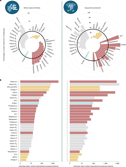
Global marine capture fisheries and aquaculture production estimates presented in this Article (Fig. 1a and Extended Data Fig. 2) were based on 208,728 and 2,507 observations, respectively. These records covered 2,304 and 492 unique species, including both fish and invertebrates, and 282 and 206 countries. Invertebrate-specific estimates for marine capture fisheries and aquaculture production (Fig. 1b and Extended Data Fig. 4) were based on 28,358 and 624 observations, covering 552 and 150 unique species and 252 and 124 countries, respectively.
Assigning nutrient composition data to aquatic foods
For each entry in the global aquatic food database, including fish and invertebrates, we assigned nutrient concentrations per 100 g and edible proportions using raw muscle-tissue samples from the AFCD12. We selected 30 nutrients with established importance for human health13: 13 minerals (calcium, chromium, copper, iodine, iron, magnesium, manganese, molybdenum, phosphorus, potassium, selenium, sodium and zinc); 11 vitamins (A, C, D, E, B1 (thiamin), B2 (riboflavin), B3 (niacin), B5 (pantothenic acid), B6, B9 (folate) and B12 (cobalamin)); five essential fatty-acid measures (total monounsaturated fatty acids (MUFAs), total omega-3 fatty acids, total omega-6 fatty acids, DHA and EPA, and ALA); and protein.
We included total protein rather than individual essential amino acids because the relevant dataset is being updated to validate units and conversion methods. Other nutrients, including cobalt and arachidonic acid, were excluded because established recommended nutrient intake (RNI) reference values were unavailable. Mean nutrient concentrations and edible proportions were assigned hierarchically according to the highest available taxonomic resolution (Supplementary Fig. 2). When species-level observations were available in AFCD, we used those values. If no species-specific measurements existed, we used the mean value from the next available taxonomic level, such as genus.
To estimate nutrient supplies, we multiplied nutrient concentrations per 100 g by equivalent live-weight production. The main analyses used live weight, which extrapolates nutrient concentrations measured in muscle tissue to total live-weight volumes. We also conducted a sensitivity analysis based on edible weight by multiplying live weight by edible proportions (Extended Data Fig. 2). Nutrient supplies and total catch or production volumes were aggregated separately for fish and invertebrates, and we calculated the percentage of total nutrient supply contributed by aquatic invertebrates. Analyses were conducted by sector, taxonomic group, year and country or exclusive economic zone (EEZ).
As observed for finfish5, country- and EEZ-level nutrient yields were not strongly correlated with the average nutrient concentration of catches (Supplementary Figs. 7 and 8). Therefore, locations with high nutrient yields did not necessarily harvest species with the highest nutrient concentrations.
Assessing the public health value of aquatic foods
We converted nutrient supplies from aquatic invertebrates into the number of annual nutrient requirements met. For each nutrient, supplies were divided by the estimated RNI averaged across available demographic groups, including sex and age categories (Supplementary Table 3). Where available, we used recommended dietary allowances61. When these were unavailable, we used adequate-intake estimates61 or values reported in the scientific literature: 433 mg per day for DHA and EPA, representing the average across reviewed studies62, and 48.8 g per day for MUFAs, equivalent to 20% of recommended total energy intake and calculated using 9 kcal per gram of MUFA63,64.
For total omega-6 fatty acids, we used recommended intake values for linoleic acids. For total omega-3 fatty acids, we used the combined recommended intake for ALA, DHA and EPA, equivalent to 1,633 mg per day. Annual nutrient supplies were divided by annual requirements after converting all values to the same units and assuming 365 days per year; for example, annual requirements in tonnes were calculated as daily requirements in tonnes multiplied by 365.
This method estimates the number of annual nutrient requirements that could theoretically be met using nutrients supplied by aquatic invertebrates alone. Although people consume diverse foods and do not depend exclusively on aquatic invertebrates for nutritional adequacy, this standardized measure enables comparisons of the public health importance of aquatic invertebrates across nutrients.
Predictive model of aquatic invertebrate nutrient concentrations
To assess variation in nutrient concentrations and identify potential drivers, we first updated and validated species-specific nutrient records for aquatic invertebrates in AFCD. We compiled, reviewed and validated 13,888 samples representing 465 invertebrate species. This process included checking source studies and food-composition tables, as well as adding information on sample preparation and relative weight.
We specifically validated the sampled food part—the body component analysed for nutrient concentration—and food processing, referring to mechanical or chemical processes that transform an animal before consumption. This included reviewing category assignments, separating processing methods from sample preparation and correcting classifications where necessary (Supplementary Table 1). Sample numbers and species coverage varied among nutrients (Supplementary Table 2).
We then linked the species-specific nutrient data with ecological and environmental traits from SeaLifeBase27. Traits were assigned hierarchically: species-level values were used when available, while missing values were replaced with the mean or most common category from the nearest available taxonomic group, such as genus. We included traits associated with energetic demand, thermal conditions, habitat and environmental setting that could influence nutrient concentrations in aquatic invertebrates (Supplementary Table 1).
Following previous research on ray-finned fishes5, we developed Bayesian hierarchical models to predict nutrient concentrations for aquatic invertebrate species from their taxonomy, ecological characteristics and environmental traits. The models also controlled for factors that could affect measurements, including sampled food part and processing method (Supplementary Table 1). Because species-specific sample sizes were limited for some nutrients (Supplementary Table 2), molybdenum and vitamins C and D were excluded from this modelling stage.
Given the hierarchical structure of the dataset and the importance of taxonomic identity in explaining nutrient variation65, taxonomy was modelled using nested random effects for samples within genus, genus within family, family within order, order within class and class within phylum. All other predictors (Supplementary Table 1) were included as fixed effects. Maximum depth was log-transformed to reduce the influence of its highly skewed distribution. Continuous predictors were standardized by subtracting the mean and dividing by twice the standard deviation. Maximum length and length at maturity were standardized within taxonomic class because different body-length measures are recorded for different invertebrate groups. Scaling by twice the standard deviation improves comparisons between continuous and binary predictors within the same model66.
Some predictors showed moderate correlations, although all Pearson correlation coefficients were below 0.6. Length at maturity was positively correlated with maximum length (Pearson correlation coefficient = 0.43), while trophic level was positively correlated with maximum depth (Pearson correlation coefficient = 0.57). These relationships indicate that larger invertebrates generally mature at larger sizes and that species at higher trophic levels tend to occur at greater depths. Although these correlations affected interpretation of marginal posterior estimates, they did not compromise model fit.
Each nutrient was modelled independently because sample sizes differed among nutrients (Supplementary Table 2). We compared three model structures using cross-validation67: a null model containing only an intercept; a hierarchical model containing taxonomic intercepts; and a full model containing the hierarchical taxonomy and ecological and environmental traits as covariates.
We initially used leave-one-out cross-validation with Pareto-smoothed importance sampling (PSIS-LOO). Because some Pareto k diagnostics were high, we also conducted k-fold cross-validation67. To enable k-fold validation, categories with few observations, such as exoskeleton food parts, were combined with broader categories, such as whole or mixed parts.
Results from k-fold cross-validation supported the leave-one-out results. For a small number of nutrients, including vitamin B12, the taxonomic hierarchy alone predicted out-of-sample data as accurately as the full model containing trait information (Supplementary Tables 5 and 6). Across nutrients, however, the full model was significantly preferred based on predictive accuracy, using the sum of leave-one-out or k-fold cross-validation information criteria under the assumption that response variables were conditionally independent. These findings supported the use of both hierarchical taxonomy and ecological and environmental traits to predict nutrient concentrations in aquatic invertebrates. The selected linear model for each nutrient was:
$$\begin{array}{l}{\mu }={\beta }_{0,\mathrm{GEN}}+{\beta }_{1}\times {\mathrm{ENVTEMP}}_{\mathrm{subtropical}}+{\beta }_{2}\times {\mathrm{ENVTEMP}}_{\mathrm{temperate}}+{\beta }_{3}\\ \,\,\times {\mathrm{ENVTEMP}}_{\mathrm{cold}}+{\beta }_{4}\times \mathrm{TL}+{\beta }_{5}\times \mathrm{DEPTH}+{\beta }_{6}\times \mathrm{LMAX}+{\beta }_{7}\times \mathrm{LM}\\ \,\,+{\beta }_{8}\times {\rm{K}}+{\beta }_{9}\times {\mathrm{ENV}}_{\mathrm{freshwater}}+{\beta }_{10}\times {\mathrm{ENV}}_{\mathrm{mixed}}+{\beta }_{11}\times {\mathrm{DEMERSPELAG}}_{\mathrm{benthopelagic}}\\ \,\,+{\beta }_{12}\times {\mathrm{DEMERSPELAG}}_{\mathrm{pelagic}}+{\beta }_{13}\times {\mathrm{DEMERSPELAG}}_{\mathrm{demersal}}\\ \,\,+{\beta }_{14}\times {\mathrm{DEMERSPELAG}}_{\mathrm{reef}}+{\beta }_{15}\times {\mathrm{DEMERSPELAG}}_{\mathrm{sessile}}\\ \,\,+{\gamma }_{1}\times {\mathrm{PART}}_{\mathrm{gills}}+{\gamma }_{2}\times {\mathrm{PART}}_{\mathrm{skin}}+{\gamma }_{3}\times {\mathrm{PART}}_{\mathrm{whole}}+{\gamma }_{4}\times {\mathrm{PART}}_{\mathrm{viscera}}\\ \,\,+{\gamma }_{5}\times {\mathrm{PART}}_{\mathrm{reptissue}}+{\gamma }_{6}\times {\mathrm{PART}}_{\mathrm{exoskeleton}}+{\gamma }_{7}\times {\mathrm{PROC}}_{\mathrm{frozen}}+{\gamma }_{8}\times {\mathrm{PROC}}_{\mathrm{dried}}\\ \,\,+{\gamma }_{9}\times {\mathrm{PROC}}_{\mathrm{canned}}+{\gamma }_{10}\times {\mathrm{PROC}}_{\mathrm{boiled}}+{\gamma }_{11}\times {\mathrm{PROC}}_{\mathrm{baked}}+{\gamma }_{12}\\ \,\,\times {\mathrm{PROC}}_{\mathrm{cooked}}+{\gamma }_{13}\times {\mathrm{PROC}}_{\mathrm{unknown}}\\ \,{\beta }_{0,\mathrm{GEN}} \sim N({\beta }_{0,\mathrm{FAM}},{\sigma }_{\mathrm{GEN}})\\ \,\,{\beta }_{0,\mathrm{FAM}} \sim N({\beta }_{0,\mathrm{ORD}},{\sigma }_{\mathrm{FAM}})\\ \,\,{\beta }_{0,\mathrm{ORD}} \sim N({\beta }_{0,\mathrm{CLASS}},{\sigma }_{\mathrm{ORD}})\\ \,\,{\beta }_{0,\mathrm{CLASS}} \sim N({\beta }_{0,\mathrm{PHY}},{\sigma }_{\mathrm{CLASS}})\\ \,\,{\beta }_{0,\mathrm{PHY}} \sim N({\beta }_{0},{\sigma }_{\mathrm{PHY}})\end{array}$$
Here, β0,…. represents estimated intercepts at different taxonomic levels: GEN, genus; FAM, family; ORD, order; CLASS, class; and PHY, phylum. These intercepts describe average continuous predictors and the most common categories for separate categorical variables, including tropical thermal regime, benthic habitat and marine environment. β0 is the global estimated intercept. β1–15 represents estimated parameters for thermal regime (ENVTEMP, subtropical, temperate or cold), trophic level (TL), maximum depth (DEPTH), maximum length (LMAX), length at maturity (LM), von Bertalanffy growth parameter (K), environment (ENV, freshwater or mixed) and preferred habitat (DEMERSPELAG, benthopelagic, pelagic, reef-associated, sessile or demersal). γ1–13 represents estimated parameters for nuisance variables, including sampled food part (PART, gills, skin, whole or multiple parts, viscera, reproductive tissue or exoskeleton) and food processing (PROC, frozen, dried, canned, boiled or steamed, baked, grilled or smoked, other cooked preparation or unknown preparation). σ… represents the standard deviation of hierarchical taxonomic intercepts.
For nutrients with few zero values (<2%; Supplementary Table 2), we used only positive observations and applied a Student’s t distribution to the natural logarithm of the nutrient concentration:
$$\log ({N}_{i}) \sim {\rm{S}}{\rm{t}}{\rm{u}}{\rm{d}}{\rm{e}}{\rm{n}}{\rm{t}}-t(\nu ,\mu ,\tau ),$$
For nutrients with more frequent zero values (Supplementary Table 2), we used a hurdle log-normal likelihood:
$$\begin{array}{l}{\rm{if}}{N}_{i}=0,\,{N}_{i} \sim {\rm{bernouilli\_logit}}\,(\delta )\\ {\rm{if}}{N}_{i} > 0,\,{N}_{i} \sim {\rm{lognormal}}\,(\mu ,\,\sigma )\end{array}$$
In these equations, Ni is the nutrient concentration in sample i; µ is the mean nutrient concentration predicted by the linear model above on the log scale; ν and τ are the degrees of freedom and scale parameters for the Student’s t distribution; δ is the estimated probability of observing a zero concentration for nutrients with more than 2% zero values; and σ is the standard deviation of the natural logarithm of the nutrient concentration.
Models were fitted in Rstan68 using the brms package69 with the following prior distributions:
$$\begin{array}{c}{\beta }_{0} \sim N(0,10)\\ \beta .. \sim N(0,2)\\ \gamma .. \sim N(0,2)\\ \nu \sim \mathrm{gamma}(2,0.1)\\ \delta \sim \mathrm{beta}(1,1)\\ \sigma .. \sim {N}^{+}(0,1)\\ \tau \sim {N}^{+}(0,1)\end{array}$$
We ran four chains for each scenario, with 10,000 iterations per chain, including 5,000 warm-up iterations and thinning by 5. This produced 4,000 posterior samples for each parameter. Convergence was assessed by starting chains from different initial values, inspecting posterior chains and distributions for stability, confirming that the potential scale reduction factor, or R hat, was close to 1 and below 1.01, and checking that effective sample sizes exceeded 400.
Because some parameters, including standard deviations for hierarchical structures, were informed by relatively small samples, we used a high number of iterations to achieve the recommended effective sample sizes. Bayesian learning was evaluated by comparing posterior and prior distributions and calculating posterior contraction values70. We assessed model fit using posterior predictive distributions and examined residual patterns against variables excluded from the model because of substantial missing data (Supplementary Figs. 5 and 10). All final models converged, represented the data adequately, showed strong posterior contraction for key parameters and produced generally well-performing probability integral transformation (PIT) plots (Supplementary Figs. 11–14).
We also used projection predictive variable selection to determine whether simpler models could outperform the full model or whether a smaller set of predictors could produce comparable results. This analysis assumed that positive nutrient concentrations followed a log-normal distribution71. The results showed that simpler subsets never achieved better predictive accuracy than the full model: the expected log predictive density of the full model was always equal to or higher than that of simpler alternatives. The predictors most important for estimating nutrient concentrations varied among nutrients. For some nutrients, removing selected covariates produced similar predictive performance, but the covariates that could be excluded differed by nutrient (Supplementary Fig. 1). Together, these findings supported the use of the full model to predict nutrient concentrations across aquatic invertebrate species.
Predicting nutrient composition for invertebrates in SeaLifeBase
We used the model parameters described above to predict nutrient composition for all macroinvertebrates recorded in SeaLifeBase27. Although SeaLifeBase likely underrepresents the full diversity of invertebrates, particularly freshwater species, it is the most comprehensive available database of life-history traits for non-fish species.
The initial database contained 71,591 species. Of these, 55,864 were classified as macroinvertebrates based on taxonomic groupings. Among them, 281 species were confirmed as edible using published sources72,73,74,75,76,77. A further 50,807 were classified as potentially edible. This group excluded 834 species known to be toxic and 4,223 species from the phyla Bryozoa, Platyhelminthes, Porifera and Priapulida. These phyla were excluded because documented human consumption was absent or biological characteristics—including chemical defences, toxicity or parasitic lifestyles—limited their suitability as food. Examples include antipredatory metabolites in bryozoans and sponges and tetrodotoxin in some flatworms.
The classification of a species as potentially edible does not indicate cultural acceptance, food safety or practical harvestability in every location. Based on available fisheries and species literature25,27,72,73, 1,083 potentially edible macroinvertebrate species were also categorized by fisheries importance as industrial, highly commercial, commercial, minor commercial, subsistence fisheries or bycatch.
We generated nutrient composition estimates for all invertebrate species, but restricted the analyses to species classified as potentially edible macroinvertebrates (Fig. 3). The database also contained ascidians from the phylum Chordata, which are technically not invertebrates. They were retained in model predictions because some share ecological and environmental traits with invertebrates and several species are consumed by humans78.
Some species lacked ecological, environmental or taxonomic information. To generate predictions for all available species, we applied several assumptions. If a taxonomic group, such as Cnidaria, lacked a group-specific estimated intercept for a particular nutrient, we used the intercept from the next higher taxonomic level, such as the global intercept, together with available ecological and trait information. When a species lacked a particular trait, we used the baseline category: the mean for continuous variables and the most common category for categorical variables, including benthic, marine and tropical.
For visualization, predicted nutrient concentrations were divided by per-capita daily RNIs. Values were capped at one when 100 g of muscle tissue supplied more than 100% of the relevant RNI. Finally, we matched predicted nutrient concentrations, expressed as RNIs, for all potentially edible macroinvertebrates with species-specific marine occurrence data35. This approach allowed us to map the geographical public health potential of aquatic invertebrates and estimate which nutrients may be available in different regions.
Aquatic invertebrate case studies
We developed six case studies covering diverse geographic regions, target species, spatial scales and management settings to demonstrate the environmental, economic, cultural and equity-related benefits of aquatic invertebrates (Fig. 4). Together, these examples illustrate how aquatic invertebrates can support nutrition indirectly by connecting ecological functions and production systems with social outcomes, including income generation, gender equality and climate resilience.
Reporting summary
Additional information about the research design is provided in the Nature Portfolio Reporting Summary associated with this Article.
Source: www.nature.com