Virtual Tissues Foundation Model Advances Multi-Scale Spatial Proteomics Analysis

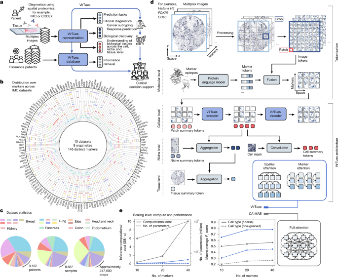
VirTues architecture for multiplexed imaging

Multiplexed imaging presents unique challenges for scalable machine learning. Unlike conventional RGB images, multiplexed tissue images contain many channels, with each channel representing a biologically distinct marker. The number and combination of markers also vary between datasets, making standard convolutional neural networks and vision transformers difficult to apply without modification.

To address these challenges, we developed VirTues, a scalable encoder–decoder foundation model based on the vision transformer (ViT) architecture. VirTues is designed to process highly multiplexed spatial imaging data with varying marker panels while preserving the biological identity of each measured protein. The model operates on image crops measuring d_c × d_c = 128 × 128 pixels. Using smaller crops increases the number and diversity of pretraining samples while reducing the computational cost of each input.

Biology-aware tokenization

VirTues uses multi-channel tokenization to preserve marker identity and support variable numbers of imaging channels^31,33. Each channel is divided into spatial patches measuring \({d}_{{\rm{p}}}\times {d}_{{\rm{p}}}=8\times 8\) pixels, approximately corresponding to the scale of a cell. After flattening, the image is represented as a token grid \({\bf{x}}\in {{\mathbb{R}}}^{M\times H\times W\times {d}_{{\rm{p}}}^{2}}\), where \(M\) is the number of measured markers and \(H=W={d}_{{\rm{c}}}/{d}_{{\rm{p}}}\).

For each measured marker, VirTues retrieves a protein embedding from a precomputed lookup table. These marker embeddings are generated with ESM-2 (ref. ¹⁸) and have dimension \({d}_{{\rm{PLM}}}=640\). The image tokens and corresponding marker tokens are projected into the shared model dimension \({d}_{{\rm{model}}}\) using learnable linear layers. The resulting tokens are fused by addition:

\({\widetilde{{\bf{x}}}}_{{mij}}={{\bf{x}}}_{{mij}}^{{\prime} }+{\pi }_{m}^{{\prime} }\).

This biology-aware tokenization allows VirTues to identify the source channel of every input token and introduces a protein sequence-based prior. Unlike one-hot marker identifiers or standard learnable embeddings, ESM-2 embeddings capture relationships between proteins and help the model generalize to markers that were not observed during training.

VirTues also introduces learnable patch summary tokens \({\bf{c}}\in {{\mathbb{R}}}^{H\times W\times {d}_{{\rm{model}}}}\). One summary token is assigned to each spatial patch, with all tokens initialized from the same weights. These tokens learn an aggregated representation of the local cellular environment.

Masked token training

During training, VirTues masks a portion of the image tokens \(\{{\widetilde{{\bf{x}}}}_{{mij}}\}\) and replaces them with a learnable masking token \({\rm{\square }}\in {{\mathbb{R}}}^{{d}_{{\rm{model}}}}\). Masking is performed independently for each channel. The masking ratio \({r}_{{\rm{masking}}}\) is sampled uniformly between 60% and 100%, and \(\lceil {r}_{\mathrm{masking}}HW\rceil \) spatial tokens are selected within each channel.

The resulting binary mask is represented by \({\bf{M}}\in \{0,1{\}}^{M\times H\times W}\), where a value of 1 identifies a masked token. Even after masking, each token remains associated with its biological marker because the corresponding marker embedding is added to the masking token.

VirTues encoder

The VirTues encoder receives all unmasked image tokens and the patch summary tokens. It modifies the standard vision transformer to efficiently process variable marker panels while learning marker relationships and spatial tissue organization separately.

Instead of computationally expensive full self-attention, VirTues alternates between two sparse attention mechanisms: marker attention and spatial attention. Marker attention connects tokens located at the same spatial position, enabling the model to learn correlations between measured proteins. For the \({\ell }\)th transformer block:

Spatial attention connects tokens from the same marker channel across different spatial positions, allowing VirTues to model tissue structure and local spatial patterns:

The encoder contains 16 transformer blocks that alternate between marker and spatial attention. Each block uses eight attention heads, two-dimensional rotary position embeddings⁷¹ and pre-layer normalization⁷². The encoder produces encoded image tokens \(\{{\mathop{{\bf{x}}}\limits^{ \sim }}_{mij}^{{\rm{e}}{\rm{n}}{\rm{c}}}\,|\,{{\bf{M}}}_{mij}=0\}\) and encoded patch summary tokens \(\{{{\bf{c}}}_{{ij}}^{{\rm{enc}}}\}\).

VirTues decoder and virtual marker generation

The VirTues decoder reconstructs masked image regions during training and can generate virtual channels during inference. It consists of a four-block ViT followed by a linear projection. For each marker channel, the decoder receives the encoded visible tokens, masked tokens and a copy of the encoded patch summary tokens:

Channels are decoded independently, preventing direct interaction between marker-specific token sets. This encourages the encoder to store meaningful biological and spatial information in the patch summary tokens. The decoder processes at most \(2{HW}\) tokens per channel, enabling full multi-head self-attention. The final reconstructed image is represented as \({{\bf{x}}}^{{\rm{rec}}}\in {{\mathbb{R}}}^{M\times H\times W\times {d}_{{\rm{p}}}^{2}}\).

To generate a new marker during inference, VirTues appends a randomly initialized channel, masks all of its tokens, supplies the target marker embedding and reconstructs the missing channel with the encoder and decoder. The asymmetric design uses a deep 16-block encoder and a lightweight four-block decoder, concentrating computational capacity in the representation-learning stage.

Cell-, niche- and tissue-level representations

During inference, VirTues represents each 128 × 128 image crop as a grid of encoded patch summary tokens \({{\bf{c}}}^{{\rm{enc}}}\in {{\mathbb{R}}}^{H\times W\times {d}_{{\rm{model}}}}\). For cell-level embeddings, the full multiplexed image is divided into overlapping crops using a 42-pixel stride. Each crop is embedded independently, and the summary tokens overlapping each cell are combined using a pixel-area-weighted average.

For niche- and tissue-level embeddings, the image is divided into non-overlapping 128 × 128 crops. Crops containing less than 30% tissue are removed. Unsupervised embeddings use mean pooling:

For supervised tasks, an attention-based multiple-instance learning classifier dynamically weights the patch tokens. The default configuration uses eight attention heads and a hidden dimension of 256.

Panoptic cell segmentation

The VirTues panoptic segmentation module contains two parallel branches: one for cell instance segmentation and one for cell type classification. Both branches use a U-Net-style decoder based on CellViT⁷³ and process intermediate patch summary tokens extracted after transformer blocks \({\ell }\in \{16,12,8,4,1\}\).

The cell typing branch predicts pixel-level class logits for \((K-1)\) cell types plus a background class:

\({{\bf{s}}}_{{\rm{celltype}}}\in {{\mathbb{R}}}^{{d}_{{\rm{c}}}\times {d}_{{\rm{c}}}\times K}\).

Softmax and argmax operations produce class probabilities and assignments. During inference, background logits are set to \(-\infty \), allowing the instance segmentation branch to determine background regions. The instance branch predicts a five-channel feature map, which is converted into cell masks using the InstanSeg⁵⁰ post-processing procedure.

Efficient attention implementation

Marker and spatial attention are implemented efficiently by merging either the channel or spatial dimension with the batch dimension. This converts each attention subset into an independent sequence and enables optimized self-attention kernels. During training, variable masking ratios and channel dropout create sequences of different lengths. To avoid padding overhead, we dynamically repackage unmasked tokens and apply block-diagonal attention masks using Flash Attention-2 (ref. ⁷⁴).

VirTues pretraining

Masked autoencoding loss

VirTues is trained end-to-end using a masked autoencoder objective^15,75. The reconstruction loss is the mean squared error between the reconstructed and original pixel intensities:

The loss is calculated over both masked and unmasked pixels.

Data augmentation

For each tissue image, we randomly sample 256 × 256 sub-images and exclude regions containing less than 30% tissue. During training, 128 × 128 crops are sampled from these sub-images. Random rotations and flips improve spatial robustness. To promote generalization across marker panels, we randomly drop between 0% and 25% of input channels for every training sample.

Pretraining optimization

VirTues is trained for 150 epochs with AdamW⁷⁶ and an effective batch size of 512. Weight decay excludes biases and layer-normalization parameters and follows a cosine schedule beginning at 0.04. The learning rate begins at 0.0002 and decays according to a cosine schedule. Training uses 16-bit automatic mixed precision and clips gradients at a maximum norm of 1.0.

Segmentation training

Segmentation and cell typing losses

Using a pretrained and frozen VirTues encoder, the instance segmentation and cell typing branches are trained jointly. The instance branch uses the InstanSeg⁵⁰ loss. The cell typing branch combines focal Tversky and cross-entropy losses.

We use \(\alpha =0.7\), \(\beta =0.3\) and \(\gamma =\frac{4}{3}\). Standard classes receive a weight of 1, while background and unknown classes receive a weight of 0.05.

Segmentation optimization

The segmentation module is trained for 100 epochs on randomly sampled crops using AdamW, an effective batch size of 64 and a learning rate of 0.001.

Datasets used to develop VirTues

Dataset curation and harmonization

We release two VirTues models: one pretrained on an imaging mass cytometry (IMC) corpus and another trained on a broader multi-technology corpus containing IMC, CODEX, Orion and MIBI data.

The IMC corpus includes 14 publicly available datasets covering lung, breast, colon, kidney, head and neck cancers, melanoma, tonsil, endometrium and healthy and diabetic pancreas. Images smaller than 256 × 256 pixels or with inadequate tissue coverage were excluded. The final IMC collection contains 8,887 images from 3,102 patients and 146 unique markers.

The extended corpus contains 32 cohorts, more than 5,100 patients and 239 protein markers across four spatial imaging technologies. Complete dataset details, including tissue origin, patient numbers, image counts, crops and annotated cells, are provided in Supplementary Tables 1 and 2.

For downstream analysis, we used cell masks, cell labels and clinical annotations from the original studies. Where necessary, labels were corrected or reannotated, including inaccurate cell labels and segmentation-mask alignment errors. Tissue masks were generated using Otsu thresholding of pixel-wise maximum projections, followed by binary opening and closing⁹⁷.

Markers were mapped to canonical UniProt protein sequences and embedded with ESM-2 (ref. ¹⁸). When multiple markers represented the same protein, the most informative marker was retained. For mRNA markers, the encoded protein sequence was used. When histone H3 was absent, a nuclear marker such as Ir191, Ir193 or Hoechst was mapped to the histone H3 sequence.

Each dataset was split into 80% training and 20% testing at the patient level, ensuring that all images from a patient remained in the same split.

Image preprocessing

Channel intensities are clipped at the 99th percentile, followed by a shifted logarithm transformation with size factor 1. Each channel is then standardized using dataset-level means and standard deviations calculated over tissue regions. Finally, images are smoothed with a Gaussian filter using a kernel size of 3 and unit variance.

Models, baselines and scaling analysis

VirTues model versions

The IMC-only VirTues model was trained on all 14 IMC datasets and used for most analyses. Additional models were trained for zero-shot evaluation, single-dataset versus multi-dataset comparisons and marker-count experiments using panels of 10, 20 and 40 markers. The multi-technology model was trained on all 32 cohorts and used to assess cross-platform generalization.

Deep learning baselines

VirTues was compared with ResNet²⁶, CA-MAE³¹ and KRONOS³⁵. ResNet embeds each channel independently using ImageNet-pretrained ResNet50 and is evaluated only for niche- and tissue-level tasks. CA-MAE uses multi-channel tokenization but lacks explicit marker identity embeddings, uses full attention and assigns a separate decoder to each channel. KRONOS is a spatial proteomics foundation model retrained on the IMC datasets where appropriate and configured with matched physical field-of-view parameters.

Marker scaling analysis

To measure how performance and computational cost change with marker number, we trained VirTues and CA-MAE on nested panels containing 10, 20 and 40 markers. Computational cost was calculated as \(c=m\times t\), where \(m\) is memory usage and \(t\) is inference time for a batch of 16 images. We also evaluated downstream macro-averaged F₁ scores for coarse and fine-grained cell classification.

VirTues evaluation

Masked image reconstruction

We evaluated VirTues reconstruction quality using independent masking, marker masking and niche masking. Independent masking tests both spatial and marker relationships. Marker masking removes every patch from one marker to assess biological marker correlations. Niche masking removes all channels at selected spatial positions to assess spatial context understanding.

Reconstruction quality was measured using Pearson correlation and mean squared error on masked pixels. Results were compared with channel-intensity inpainting and predictions based on the most correlated visible marker. For zero-shot marker reconstruction, we related performance to the L2 distance between the new marker’s ESM-2 embedding and its three nearest pretrained markers.

Cell-level phenotype classification

Because VirTues patch summary tokens capture information at cellular scale, we evaluated them using cell phenotype classification across six datasets. Linear probes used logistic regression with an L-BFGS solver and L2 regularization. The same patient-level train–test split was used for all methods. Performance was reported using class-specific and macro-averaged F₁ scores with bootstrap confidence intervals.

• Coarse cell typing of Cords et al.⁴²: six classes, including tumour, fibroblast, immune, T cell, vessel and other.

• Fine-grained cell typing of Cords et al.⁴²: 22 classes covering immune, stromal, vascular and tumour phenotypes.

• Cell typing of Danenberg et al.⁶: eight classes, including natural killer, B, T, myeloid, stromal and APC populations.

• Cell typing of Hoch et al.⁴⁸: tumour, lymphocyte, macrophage, stroma, T cell and other classes.

• Coarse and fine-grained cell typing of Wang et al.², including immune, stromal, tumour, vascular and T-cell phenotypes.

• Cell typing of Phillips et al.⁴⁴: tumour, epithelium, myeloid, stroma, T, vascular, B, Langerhans, mast, nerve and neutrophil classes.

• Cell typing of Lin et al.⁴: tumour, endothelial, stromal, vascular, B-cell, T-cell, macrophage and related classes.

We also tested whether cell typing remained stable after replacing measured markers with VirTues-generated virtual markers. Key B-cell and T-cell markers were progressively removed, reconstructed and used for renewed phenotype classification.

Cross-cohort cell segmentation and typing

To evaluate cross-cohort generalization, cell labels from ten datasets were harmonized into tumour, fibroblast/stroma, myeloid, CD8 T cell, CD4 T cell, B cell, vessel/endothelial and unknown categories. A separate segmentation module was trained for each evaluation dataset while excluding that dataset from training.

Instance segmentation was evaluated using F₁ scores at multiple intersection-over-union thresholds and compared with Cellpose⁴⁹, InstanSeg⁵⁰ and StarDist⁵¹. Cell typing was evaluated using macro-averaged F₁ scores and compared with MAPS⁵⁴ and Astir⁵⁵.

Tissue structure and patient risk stratification

Using the METABRIC-derived dataset of Danenberg et al.⁶, we represented each tissue using cell summary tokens and clustered them into 120 cellular states. Each tissue was then represented by a cluster-proportion vector and grouped into four structural classes. These classes were merged into high- and low-risk groups according to survival outcomes. Kaplan–Meier curves, log-rank tests and risk ratios were used to assess survival differences and associations with known tumour microenvironment structures.

Tissue-level classification

We evaluated VirTues embeddings on clinically relevant tissue-level tasks, including cancer subtype, relapse, tumour grade, ERBB2 status, oestrogen receptor status, PAM50 subtype and treatment response. Gated ABMIL classifiers aggregated patch-level representations using eight attention heads with a hidden dimension of 256.

1. (a)

   Cancer subtype: adenocarcinoma or squamous cell carcinoma.

2. (b)

   Relapse: relapse or no relapse.

3. (c)

   Grade: Grade 1, Grade 2 or Grade 3.

1. (a)

   ERBB2 status: ERBB2⁺ or ERBB2⁻.

2. (b)

   Oestrogen receptor status: receptor-positive or receptor-negative.

3. (c)

   PAM50 subtype: normal-like, Basal, HER2, Luminal A or Luminal B.

4. (d)

   Grade: Grade 1, Grade 2 or Grade 3.

1. (a)

   Treatment response: pathological complete response or residual disease.

Models were trained with Adam⁷⁶, a learning rate of 10⁻⁴, a batch size of 16 and early stopping. Performance was averaged across five runs and compared with KRONOS³⁵, CA-MAE³¹ and ResNet²⁶.

Zero-shot inference on new datasets

Zero-shot generalization was assessed using leave-one-dataset-out training. Separate VirTues models were trained without one selected dataset and then evaluated on that unseen dataset. Tasks included masked reconstruction and cell-type classification. Reconstruction was evaluated for both familiar markers and markers never observed during pretraining.

Information retrieval using spatial tissue embeddings

VirTues can retrieve tissues with similar molecular and spatial phenotypes. Rather than compressing an entire tissue into a single vector, we represented each patient using multiple niche-level embeddings. Similarity between tissues was measured using the 2-Wasserstein distance:

Retrieval quality was assessed using cell-type composition and sliced Wasserstein distance between pixel-level molecular profiles:

Clinical feature matching was compared with randomized retrieval using two-sided McNemar tests. Confidence intervals were estimated by bootstrap resampling over query tissues.

Quantifying treatment response

We used the breast cancer dataset of Wang et al.², which includes samples collected before, during and after treatment. The analysis focused on patients receiving both chemotherapy and immunotherapy with available pre- and on-treatment biopsies. Treatment response was quantified using the entropy-regularized 2-Wasserstein distance between cell-level representations:

We used \(\varepsilon ={10}^{-3}\) and compared response distances between responders and non-responders with two-sided Mann–Whitney U tests. UMAP and Wasserstein barycentres were used to visualize changes in cellular-state distributions over time:

Foundation model biomarkers for therapy response

To identify virtual spatial biomarkers associated with immunotherapy response, we analyzed pretreatment samples from 111 patients. Cell summary tokens were clustered with Leiden clustering across multiple resolution settings. Clusters containing fewer than 2,000 cells were retained, and each patient–cluster pair was represented using four ordinal abundance ranks.

Univariate logistic regression and repeated stratified cross-validation were used to calculate AUROC values. The highest-performing response and non-response clusters were selected as virtual spatial biomarkers. Their combined predictive value was evaluated with multivariate logistic regression and compared with previously reported spatial predictors and tumour-to-immune-cell ratios.

We further characterized the cellular composition of each predictive cluster and measured neighbouring cell-type distributions to improve biological interpretation.

Cross-cohort validation of spatial biomarkers

To test translational robustness, the VirTues-derived spatial biomarkers were transferred to an independent triple-negative breast cancer cohort from Meyer et al.³. The validation cohort was not used for VirTues pretraining or biomarker discovery.

Random forest classifiers trained on Wang et al.² cell embeddings predicted membership in response and non-response clusters in the independent cohort. Patients were assigned risk scores based on the abundance of these clusters and divided into high-, medium- and low-risk groups. Kaplan–Meier survival analysis, log-rank testing and concordance indices were used to evaluate disease-free survival.

VirTues model inspection and visualization

We examined attention patterns to assess whether VirTues learns biologically meaningful marker and spatial relationships. Marker-attention scores from the first encoder layer were aggregated across attention heads and spatial positions to generate marker importance scores:

To visualize spatial attention, we added learnable channel summary tokens positioned at the centre of the input crop. The augmented model was fine-tuned for cancer subtype prediction, and attention from the channel summary token to patch summary tokens was displayed as a spatial heatmap.

Computing hardware and software

Experiments were implemented in Python 3.12.9 using PyTorch 2.5.1, CUDA 12.1 and Flash Attention-2 2.7.4. Additional software included NumPy, zarr, pandas, matplotlib, seaborn, fair-esm, scikit-image, scikit-learn, scikit-survival, lifelines, cuML, instanseg-torch, napari, wsireg and QuPath. Pretraining was performed on NVIDIA GH200 GPUs in a high-performance computing environment. Downstream experiments used NVIDIA A100 80 GB GPUs.

Reporting summary

Additional information about the research design, datasets, statistical methods and reporting standards is available in the Nature Portfolio Reporting Summary linked to this article.