


Experimental Setup and Spectroscopy of Ising and Tricritical Ising CFTs in a Rydberg Atom Quantum Simulator
Experimental Setup for the Rydberg Atom Quantum Simulator
A detailed description of the experimental apparatus has been reported previously.35,60,61 In summary, individual 88Sr atoms are trapped in a programmable one-dimensional array of optical tweezers operating at 813 nm. Acousto-optic deflectors (AODs) generate and control the tweezer array, enabling precise manipulation of the atom positions and system size.
The atoms are initially prepared in the 5s2 1S0 state and cooled on the narrow-line red transition 5s2 1S0 ↔ 5s5p 3P1 at 689 nm. This cooling process brings the atoms close to their motional ground state. The atoms are then rearranged into a defect-free array with the desired number of sites.
After rearrangement, the atoms are transferred to the metastable clock state 5s5p 3P0 using a direct π pulse at 698 nm combined with incoherent optical pumping.60 For system sizes of L = 26, 27 and 35, up to two rounds of dark-state-enhanced loading are used to improve defect-free state-preparation fidelity. The number of available tweezers is limited primarily by laser power.62
In the quantum simulator, the metastable clock state 5s5p 3P0 represents the computational ground state, denoted by |0⟩. It is coupled to the Rydberg state 5s61s 3S1, denoted by |1⟩, through a single-photon transition at 317 nm.
Following evolution under the Hamiltonian in equation (1), a 408 nm auto-ionization beam removes atoms occupying the Rydberg state.35 The remaining atoms are subsequently optically pumped out of the clock state and detected through fluorescence on the 5s2 1S0 ↔ 5s5p 1P1 transition at 461 nm.63
Interaction Parameters at the Ising and TCI Critical Points
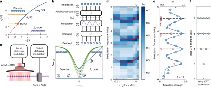
For the two Ising conformal field theory (CFT) configurations, corresponding to configurations (1) and (2) in Fig. 4, the data shown in Figs. 1–3 and Fig. 4b are collected using a Rydberg Rabi frequency of Ω = 2π × 6.0 MHz. The exception is Fig. 1d, where Ω = 2π × 7.5 MHz.
For the Ising transition, the next-nearest-neighbour interaction is V2 = 2π × 3.06(1) MHz, with a lattice spacing of a = 3.3 μm. The measured nearest-neighbour interaction is V1 = 2π × 164.6(9) MHz at the same spacing.
For the tricritical Ising (TCI) point, the experiment uses Ω = 2π × 5.5 MHz, V2 = 2π × 8.96(15) MHz and a lattice spacing of a = 2.8 μm. The critical detunings for configurations (1), (2) and (3) are, respectively, Δc = 2π × 10.2 MHz, −0.9 MHz and −8.3 MHz.
Post-Selection and Experimental Data Quality
Experimental data are filtered using a four-stage post-selection protocol designed to remove shots that do not accurately represent the intended quantum system.
- Defect-free rearrangement: Only experimental shots containing a defect-free array with the correct system size are retained.
- Erasure detection: Erasure imaging is performed twice: once after initial state preparation and again after the Rydberg pulse.60 Atoms detected in the 5s2 1S0 state have leaked outside the qubit subspace, so those shots are discarded.
- Rydberg blockade filtering: Because the experiment operates in the blockade regime, where V1 ≫ V2, Ω and Δ, simultaneous nearest-neighbour Rydberg excitations are strongly suppressed. Shots with no detected atom on consecutive sites after the Rydberg pulse are removed. This procedure also filters out atom loss that is not distinguishable from Rydberg occupation during readout.
- Rydberg-pulse verification: The Rydberg laser pulse is monitored with a photodiode and recorded on an oscilloscope. Approximately 0.6% of shots have no detectable pulse because the arbitrary waveform generator failed to produce the programmed radiofrequency waveform. These shots are discarded.61
Depending on the measurement, between 20% and 70% of the experimental runs remain after post-selection.
Adiabatic State Preparation and Backward Sweeps
For adiabatic state preparation, the Rabi frequency and detuning of the global Rydberg beam are modulated with AODs. At the operating magnetic field of B = 70 G, the Rydberg interaction is repulsive, so Vij > 0.
The global detuning begins at a large negative value and is increased toward the critical point using a tangent-shaped time profile. This profile slows the sweep near criticality and improves preparation of the ground state. Starting with all atoms in |0⟩, the protocol prepares the many-body ground state at the critical point.
To access the effective attractive-interaction sector, where Vij < 0 for |i − j| ≥ 2, the signs of the Hamiltonian terms are reversed by changing the detuning relative to the critical value, Δ − Δc. Because V1 is much larger than the remaining energy scales, the eigenstates separate into sectors divided by approximately V1. The highest-energy state in the blockade-preserving sector of the native Hamiltonian corresponds to the ground state of the sign-reversed blockade Hamiltonian. This preparation protocol is referred to as a backward sweep.
After the sweep, the detuning is either held at the critical point for σ-field measurements or ramped symmetrically into the ℤ2-ordered or disordered phase for spectroscopy. The ramp parameters are optimized to minimize residual excitations.
Local Detuning Control and Tweezer-Induced Light Shifts
Experiments requiring site-dependent detunings δΔi use the same 813 nm optical tweezers that provide atom confinement. When local detuning control is unnecessary, the tweezer light is rapidly switched off with an acousto-optic modulator before the Rydberg pulse.64 This reduces detuning noise caused by tweezer-intensity fluctuations and prevents anti-trapping of the Rydberg state.
The tweezer light produces a tunable light shift on the 5s5p 3P0 ↔ 5s61s 3S1 transition. For a tweezer power of 1.4(2) mW per site and a waist of 0.75(5) μm, the measured light shift is −3.545(54) MHz. At this intensity, the atom-loss time constant caused by Rydberg-state anti-trapping is 63(12) μs.
Local detunings are calibrated for every tweezer configuration with a Ramsey sequence before data acquisition. Extended Data Fig. 5 shows an example for L = 26 at the tricritical point with fixed boundary conditions.
Determining the Ising and TCI Critical Points
Finite-Size Scaling of the Ising Critical Point
The parameters required to prepare the system on the Ising critical line are determined through exact diagonalization of the effective Hamiltonian in equation (1). The analysis uses the second-order PXP Hamiltonian derived through a Schrieffer–Wolff transformation.65 With δΔi = 0, the interaction coefficients are
$${V}_{ij}=\left\{\begin{array}{ll}{V}_{1} & |i-j|=1\\ \frac{64{V}_{2}}{|i-j|^{6}} & |i-j|\ge 2.\end{array}\right.$$
The second-order correction is
$${\hat{H}}_{2}=-\frac{{\Omega}^{2}}{4{V}_{1}}\left[\sum_i\left(2{\hat n}_i-\frac{3}{2}{\hat n}_{i-1}{\hat n}_{i+1}+({\hat P}_{i-1}{\hat b}_{i}^{\dagger}{\hat b}_{i+1}{\hat P}_{i+2}+\mathrm{h.c.})\right)\right],$$
where \({\hat b}_{i}=|0\rangle_i\langle1|_i\) is the hard-core boson operator.
Following the curve-crossing method, the central observable is the ground-state expectation value of the order parameter in the middle of the chain, \(\langle\hat{\sigma}_{L/2}\rangle\). For each system size and detuning, we analyze the rescaled quantity
$${\sigma}_{\mathrm{RS}}=\langle{\hat{\sigma}}_{L/2}\rangle\sin\left(\frac{\pi}{L+2}\right)^{-1/8}.$$
The crossing point obtained through finite-size scaling identifies the critical detuning in the thermodynamic limit. Extended Data Fig. 2a presents this analysis for V2/Ω = ±0.51.
Locating the Tricritical Ising Point
Locating the TCI point requires varying two Hamiltonian parameters simultaneously. For a fixed interaction strength V2, the energy ratios Ei/E1 are calculated for several detunings and system sizes. The crossing of curves for system sizes L − 1 and L + 1 determines both the crossing detuning ΔX and the corresponding energy ratio.
These values are extrapolated to the thermodynamic limit and compared with the free-boundary TCI spectrum, whose low-energy ratios are 3:4:5:6:7:8:…. At V2/Ω = −1.63, the calculated ratios E2/E1 and E3/E1 agree most closely with 4/3 and 5/3. The critical detuning is then determined as Δc/Ω = −1.51.
Coherent Control of Many-Body Quantum States
Modulation spectroscopy can coherently transfer population from a many-body ground state to a selected excited state. When the modulation frequency matches the energy difference between the states, the system undergoes many-body Rabi oscillations.
Let |g⟩ denote the ground state and |e1⟩ the first excited state. The Hamiltonian can be written as
$${\hat H}=E_g|g\rangle\langle g|+(E_g+E_1)|e_1\rangle\langle e_1|+\cdots.$$
A weak modulation of the form \(\delta\hat H=A\cos(E_1t+\varphi)\hat K\) produces an effective two-level Hamiltonian in the rotating frame. The many-body Rabi frequency is
$${\Omega}_{\mathrm{MB}}=A|\langle g|\hat K|e_1\rangle|.$$
In a seven-atom array, the atoms are initialized in |0⟩ and adiabatically ramped to Δ = 2π × 8.8 MHz, slightly away from criticality. A global detuning modulation with frequency ω = 2π × 2.83 MHz is then applied for a variable duration t.
The ground and first excited states are transferred into the ordered states |1010101⟩ and |1001001⟩, respectively. The measured observable is
$${\hat O}’=\sum_i(1-\hat n_i),\qquad \delta n=\langle{\hat O}’\rangle-3.$$
Thus, δn = 0 corresponds to the ground state and δn = 1 to the first excited state. The experiment observes coherent oscillations with a frequency of 0.506(5) MHz, an initial contrast of 0.83(3) and a 1/e coherence time of 5.5(5) μs.
Ramsey Interferometry and Many-Body Phase Coherence
To measure the first excitation energy accurately and determine the coherence time, the experiment uses Ramsey interferometry. After preparing the ground state, a π/2 pulse creates the superposition
$$\frac{|g\rangle+|e_1\rangle}{\sqrt{2}}.$$
The modulation is then switched off, allowing the superposition to evolve under the Hamiltonian for a controlled time. The resulting phase evolution directly reveals the energy difference E1 and provides a measurement of many-body phase coherence.
Modulation–Ramp–Probe Spectroscopy
In modulation–ramp–probe spectroscopy, a weak time-dependent perturbation transfers population from the ground state to excited states. Because the measurement observable is diagonal in the eigenbasis of the critical Hamiltonian, the response is quadratic in the modulation amplitude.
For a Gaussian modulation envelope, the measured response is a sum of Gaussian peaks centered at the excitation energies:
$$\delta\langle\hat O\rangle=\frac{\pi w^2A^2}{4}\sum_e(O_{ee}-O_{gg})|K_{ge}|^2
e^{-\frac{w^2}{2}(\omega-\Delta E_{eg})^2}.$$
Here, ΔEeg = Ee−Eg, Kge = ⟨g|\(\hat K\)|e⟩ and Oee and Ogg are diagonal matrix elements of the measurement operator.
The observable is chosen as \({\hat O}’=\sum_i(1-\hat n_i)\) because it is robust against common-mode atom loss and distinguishes the ground state from excited states.
After modulation, the detuning is adiabatically ramped into either the disordered or the ℤ2-ordered phase. In these limits, the measurement operator becomes diagonal in the eigenbasis of the final Hamiltonian. The adiabatic ramp therefore maps the original eigenstates to distinguishable measurement states without changing their populations.
For odd chains, ramping into the ℤ2 phase is advantageous because the ordered ground state remains unique and the first excited manifold has a larger degeneracy. For even chains, the ordered ground state is degenerate, so the system is ramped back into the disordered phase for spectroscopy.
Modulation–Probe Measurements and the Dynamical Structure Factor
The modulation–probe sequence measures the linear response of an observable \(\hat Q\) that is not necessarily diagonal in the eigenbasis of the Hamiltonian. The response contains products of transition matrix elements such as KgeQeg and is therefore linear in the modulation amplitude.
For a thermal initial state, the linear response at modulation frequency ω is
$$\delta\langle\hat Q\rangle(\omega)=\frac{\sqrt{2\pi}A}{Z}
\sum_{m,n}(e^{-\beta E_m}-e^{-\beta E_n})
\mathrm{Im}[Q_{mn}K_{nm}F(\omega-(E_n-E_m))
e^{i(E_m-E_n)T}e^{-i\varphi}].$$
In the continuum limit, the response becomes proportional to the dynamical structure factor. By selecting
$$\hat Q=\sum_j e^{-ikj}\hat o_j,\qquad \hat K=\hat Q^\dagger,$$
the measured signal directly probes momentum- and frequency-dependent excitations.
To suppress unwanted even-order responses, measurements are performed with modulation phases φ and φ + π. Even-order terms are unchanged under this phase shift, whereas the linear response changes sign. Subtracting the two signals therefore cancels the dominant quadratic response while preserving the linear component.
Definition of the Dynamical Structure Factor
The dynamical structure factor describes the spatial and temporal correlations of a quantum system and encodes the momentum and frequency distribution of its excitations. For a local field operator \(\hat o_i\), it is defined as
$$S(k,\omega)=\frac{1}{LZ}\sum_{j,l}\int_{-\infty}^{\infty}dt\,
e^{-ik(j-l)+i\omega t}
\mathrm{Tr}[e^{-\beta H}\hat o_j(t)\hat o_l(0)].$$
With the modulation phase chosen as ωT+φ = −π/2, the continuum response satisfies
$$S(k,\omega)=\frac{1}{\pi f(T^-)AL(1-e^{-\beta\omega})}
\delta\langle\hat Q\rangle^{\mathrm{cont.}}(\omega).$$
This relationship shows that modulation–probe spectroscopy provides a direct experimental measurement of the dynamical structure factor.
Ising CFT and TCI Excitation Spectra
Low-Energy Ising Excitations
The second-order Ising phase boundary is described at low energies by right- and left-moving Majorana fermions, γR(x) and γL(x). The effective Hamiltonian for an open chain of length L is
$${\mathcal H}_{\mathrm{Ising}}=\int_{-L/2}^{L/2}dx
\left(-i\hbar v\gamma_R\partial_x\gamma_R+
i\hbar v\gamma_L\partial_x\gamma_L\right).$$
Open-boundary conditions quantize the momenta according to
$$k_n=\frac{\pi}{L}\left(n+\frac{1}{2}\right),\qquad n\in\mathbb Z,$$
with excitation energies \(\hbar vk_n\). The boundary conditions produce anti-periodic fermionic modes and prevent the appearance of an unphysical isolated Majorana zero mode.
For odd-length chains, the physical states contain an even number of fermionic excitations. For even-length chains, the boundary conditions require an odd number of fermions. This even–odd effect determines which conformal towers appear in the measured spectrum.
The Ising CFT has central charge c = 1/2 and primary fields with chiral scaling dimensions 0, 1/16 and 1/2. The corresponding finite-size energy levels are
$${E}_{\alpha,J}\sim\frac{\pi\hbar v}{L}
\left(h_\alpha+J-\frac{c}{24}\right),\qquad J\ge0.$$
Tricritical Ising Excitations
The TCI point is described by a strongly interacting conformal field theory with central charge c = 7/10. Its six primary fields have chiral dimensions
0, 3/80, 1/10, 7/16, 3/5 and 3/2.
The leading charge-density-wave order parameter has scaling dimension 3/40. The two symmetric relevant fields have dimensions 1/5 and 6/5 and drive the system away from the TCI point.
Boundary conditions determine the conformal towers present in the spectrum. Fixed boundary conditions produce the identity tower for odd chains and the ε″ tower, beginning at scaling dimension 3/2, for even chains. Free boundary conditions produce both the identity and ε″ towers.
Momentum-Dependent Modulation Spectroscopy
For open chains, momentum is not a strict quantum number because translation symmetry is broken. Nevertheless, spatially varying modulation reveals a characteristic dependence on the wavevector k and directly exposes the linear dispersion of the Ising CFT.
The momentum-dependent modulation operator is
$$\hat K_k\sim i\int_{-L/2}^{L/2}dx\,
\cos(kx+\alpha)\gamma_R(x)\gamma_L(x).$$
For reflection-symmetric modulation profiles, α = 0 or π, the ground state couples primarily to even-reflection-parity excited states. For reflection-antisymmetric profiles, α = ±π/2, the response selects odd-reflection-parity states.
The transition amplitude is strongest when
$$|k|=|k_a-k_b|=\frac{|a-b|\pi}{L},$$
where ka and kb are the momenta of the two excited fermions. The corresponding excitation energy is approximately
$$E\simeq\hbar v|k|+O(L^{-1}).$$
This result produces a light-cone-like dispersion relation. Scanning the modulation wavevector can also distinguish states that are degenerate in energy but have different momentum differences.
Dynamical Structure Factor and Universal CFT Scaling
The imaginary-time correlation function of a field \(\hat\phi\) is
$$C(x,\tau)=Z^{-1}\mathrm{Tr}
[e^{-\beta H}\hat\phi(x,\tau)\hat\phi(0,0)].$$
For a scalar primary field with scaling dimension Δφ, the thermodynamic-limit correlation function follows the universal form
$$C(x,\tau)\sim(x^2+v^2\tau^2)^{-\Delta_\phi}.$$
After Fourier transformation and analytic continuation, the zero-temperature dynamical structure factor scales as
$$S(k,\omega)\propto
(\omega^2-v^2k^2)^{\Delta_\phi-1}
\theta(|\omega|-v|k|).$$
For the Ising CFT, the energy field ε has Δε = 1, while the order parameter σ has Δσ = 1/8. Therefore,
$${S}_{\varepsilon}(k,\omega)\propto
\theta(|\omega|-v|k|),$$
and
$${S}_{\sigma}(k,\omega)\propto
(\omega^2-v^2k^2)^{-7/8}
\theta(|\omega|-v|k|).$$
At k = 0, the ε-field structure factor is constant above the light-cone threshold. At k = 0, the σ-field response decreases approximately as ω−7/4. These scaling laws provide an experimentally accessible signature of Ising CFT universality.
Analysis of Measured Spectra
Excited-state energies are extracted from modulation–ramp–probe measurements by fitting the measured response to a sum of Gaussian peaks:
$$\delta n(f)=a_0+\sum_i a_i
\exp\left[-\left(\frac{f-E_i/h}{w_i}\right)^2\right].$$
The fitted positive-frequency centres Ei are interpreted as excitation energies relative to the ground state. For shorter modulation times, both positive- and negative-frequency contributions are included in the fitting function.
Optimal parameters are obtained by minimizing
$$\chi^2=\sum_j
\frac{[\delta n_{\exp}(f_j)-\delta n_{\mathrm{model}}(f_j)]^2}
{\sigma_j^2},$$
where σj is the statistical uncertainty at frequency fj. Parameter uncertainties are determined by bootstrap resampling using normal distributions centred on the measured data.
For system sizes L ≥ 19, the measured critical spectra agree with the Ising CFT prediction within 3σ. The reduced chi-square is χ2/ν = 0.98, supporting the conclusion that the critical Rydberg chain is described by the Ising CFT.
Numerical Simulation of the Linear Response
The lattice representation of the Ising energy field is
$${\hat\varepsilon}_{i+1/2}={\hat n}_i+{\hat n}_{i+1}.$$
Consequently, global detuning modulation realizes a zero-wavevector ε-field modulation:
$$\hat K=\sum_i\hat n_i=\frac{1}{2}\sum_i\hat\varepsilon_i.$$
After applying the global modulation, all local Rydberg occupations \(\hat n_i\) are measured to reconstruct the response of the ε-field operator.
Experimental observations are compared with tensor-network simulations based on matrix product states. The ground state is obtained using the density matrix renormalization group, while time evolution under the time-dependent Hamiltonian is calculated using the time-dependent variational principle.
For efficient numerical calculations, interactions are truncated to distances |i−j| ≤ 2, resulting in the simplified Hamiltonian
$${\hat H}=\frac{\Omega}{2}\sum_i
\hat P_{i-1}\hat X_i\hat P_{i+1}
-\Delta\sum_i\hat n_i
+V_2\sum_i\hat n_i\hat n_{i+2}.$$
Tweezer-induced light shifts are compensated with a synchronized global detuning modulation. This allows the experiment to create controlled spatial modulation patterns for probing both ε- and σ-field dynamical structure factors.
Quench Dynamics Near the TCI Point
In addition to equilibrium spectroscopy, the experiment investigates nonequilibrium dynamics near the tricritical Ising point. Because the TCI spectrum contains rational energy ratios, a low-energy state can exhibit periodic revivals and oscillations.
The experimental protocol begins with adiabatic preparation near the TCI point, followed by a sudden quench of the detuning to Δc. The system is held at criticality for a variable time, after which the sum of local order-parameter fields is measured.
Numerical simulations predict long-lived oscillations for local detuning strengths η between 0 and 1. The fitted oscillation frequencies are consistent with the first excited-state energy E1, indicating coherent oscillations between the ground state and the first excited TCI state.
Experimentally, damped oscillations are observed for boundary detunings η = 0.5 and 0.75. The measured frequencies show qualitative agreement with numerical predictions, although uncertainties in V2 and rapid decoherence limit the precision.
The observed damping is attributed primarily to laser noise, decoherence and shot-to-shot fluctuations in the interaction strength. Improved noise suppression and more accurate calibration of V2 should extend the coherence time. Together with modulation spectroscopy, the quench measurements provide additional evidence that the experiment reaches and probes the TCI critical point.
Conclusion
This Rydberg atom quantum simulator provides a flexible platform for studying quantum criticality, conformal field theory and nonequilibrium many-body physics. Programmable strontium atom arrays enable precise control of interactions, detunings, boundary conditions and modulation wavevectors.
Using adiabatic preparation, coherent many-body control, Ramsey interferometry and modulation spectroscopy, the experiment measures Ising and tricritical Ising excitation spectra. The observed energy levels, reflection properties, light-cone dispersion and dynamical structure-factor scaling are consistent with universal CFT predictions.
These results demonstrate how quantum simulators can access both individual finite-size excitations and continuum response functions, providing a direct experimental route to universal quantum-field-theory phenomena.
Source: www.nature.com