


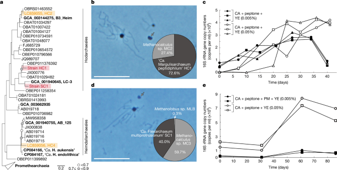
The study combined environmental sampling, anaerobic cultivation, molecular biology, microscopy, chemical analysis and comparative genomics to investigate Promethearchaeota strains from a Japanese gas field. Researchers collected biofilms from the KTG3 gas-production well, isolated and monitored the HC1 and SC1 cultures, characterized their cells and growth, and analysed their genomes, transcripts, proteins and glycoproteins. Phylogenetic and metabolic analyses were then used to examine Promethearchaeota evolution and their potential for peptide degradation and aerobic or oxygen-tolerant metabolism.
Sample collection and cultivation
Biofilm samples were collected from the KTG3 gas-production well in the Southern Kanto gas field, Chiba Prefecture, Japan. The biofilm grew on the wall of a separator discharge outlet 20–40 cm below the water surface. Samples were collected after brine eruptions on 29 August 2019, 16 July 2020 and 11 May 2023 (Extended Data Fig. 1).
The gas field lies in an ancient marine forearc basin containing subsurface gas reservoirs in turbidite sandstones, making it geologically and geochemically relevant to past seawater and marine sediments66. Brine from KTG3 is rich in organic matter, iodine and iron. Further site information has been reported previously37, and the brine’s geochemical characteristics are shown in Extended Data Fig. 1b.
Collected biofilm was placed in a 100 ml glass bottle filled completely with brine and transported to the laboratory under refrigeration. Samples were also inoculated at the site into 50 ml glass vials containing anaerobic medium (Supplementary Note 2). iTag analysis showed that the biofilm contained abundant and diverse microorganisms, most of them affiliated with uncultured or difficult-to-cultivate groups, including Promethearchaeota.
To isolate new Promethearchaeota strains, the researchers used strategic batch cultivation35 informed by previous knowledge and expectations about this archaeal group (Supplementary Note 1). Details of the media, cultivation procedures and purity checks for the HC1 and SC1 cultures are provided in the Supplementary Methods.
Unless otherwise stated, HC1 was grown in medium containing casamino acids, peptone and yeast extract, each at 0.005% (w/v). SC1 was grown in medium containing casamino acids, powdered milk, polypeptone peptone and yeast extract at 0.005%, 0.005%, 0.01% and 0.05% (w/v), respectively. The inoculum represented 16% (v/v) of HC1 cultures and 20% (v/v) of SC1 cultures.
Dissolved oxygen in KTG3 culture medium without reducing agents was measured using a fibre-optic oxygen meter (Fibox 3 trace, Presence) and an SP-PSt6-YAU oxygen sensor. The sensor was attached to the inner wall of 50 ml serum bottles with oxygen-permeable silicone adhesive.
Growth monitoring and temperature and substrate experiments
DNA extraction, PCR-mixture preparation and quantitative PCR (qPCR) were performed as described previously4,67. qPCR primers were designed with the probe-design tool in the ARB program68. Primer specificity was checked using BLAST and the ARB-SILVA database (https://www.arb-silva.de/)69. Primer sequences and PCR conditions are listed in Supplementary Table 23.
Doubling times were calculated from semilogarithmic plots of qPCR data. For iTag analysis, the researchers used the universal primer pair 530F/907R, which included 5′ overhang adapters70. Library construction, sequencing and data analysis followed previously described procedures4. All samples used for data acquisition were checked for growth and microbial composition by qPCR and iTag analysis before or after the experiments.
To assess temperature ranges, a pure HC1 co-culture and an SC1 tri-culture were incubated from 10 °C to 45 °C and from 10 °C to 50 °C, respectively. Each condition was tested in triplicate. After incubation, qPCR was used to measure the 16S rRNA gene copy number of each strain.
Substrate use was tested by supplementing basal media with individual substrates sterilized by autoclaving or filtration. Two successive transfers were made under the same cultivation conditions, and qPCR targeting the strains’ 16S rRNA genes was performed on both the first and second subcultures. These experiments were conducted in duplicate at each strain’s optimum growth temperature.
To test non-proteinaceous substrates, individual substrates were added to HC1 medium containing casamino acids, peptone and yeast extract, or to SC1 medium containing casamino acids, powdered milk, polypeptone peptone and yeast extract. Each condition was tested in duplicate.
Microscopy and cell-size measurements
Epifluorescence microscopy
Routine observations used an epifluorescence microscope (BX53, EVIDENT) equipped with a phase-contrast objective and a colour CCD camera system (DP80 or DP75, EVIDENT). Images were acquired and recorded with cellSense v.4.3 (EVIDENT). Agarose-coated glass slides were used when images had to be captured without cell movement caused by Brownian motion71. HC1 cell and protrusion diameters were measured from phase-contrast images with Fiji, an image-analysis package based on ImageJ72.
Scanning electron microscopy
For scanning electron microscopy (SEM), archaeal cells were fixed with 2.5% (w/v) glutaraldehyde for 2 h under anoxic conditions at their optimum growth temperatures, followed by overnight fixation at 4 °C. Sample preparation followed a previously described protocol3. Samples were examined with an extreme-high-resolution focused ion beam SEM (FIB-SEM; Helios G4 UX, Thermo Fisher Scientific) operated at 1 kV.
To measure the volumes and numbers of HC1 cell bodies, protrusions and membrane vesicles at different yeast-extract concentrations, wide-area SEM images were acquired with Maps v.2.5 (Thermo Fisher Scientific). Each wide-area image was assembled from 100 images in a 10 × 10 arrangement. Individual images were acquired at 1 kV with a 13 pA beam current, a 36.3 µm × 24.2 µm field of view and a resolution of 23.6 nm per pixel.
Images were analysed with AMIRA 3D Pro 2024.1 and 2024.2 (Thermo Fisher Scientific). They were first denoised by curvature-driven diffusion73. HC1 cell bodies, protrusions, membrane vesicles and Methanocalculus cells were segmented with a deep-learning module based on PyTorch74 and Keras (https://github.com/fchollet/keras). A model trained on 2,000 × 2,000-pixel images was adapted to the full images, followed by manual correction and watershed segmentation.
Each segmented component other than protrusions was labelled, and its area and perimeter were measured. Protrusions were skeletonized with the Auto Skeleton module75. Researchers measured the number of fibre segments and their curved lengths after excluding looped fibres and fibres shorter than 10 pixels.
Transmission electron microscopy
Ultrathin sections of archaeal cells were prepared using a previously established protocol3. Sections were examined with a conventional transmission electron microscope (Tecnai 20, FEI) operated at 120 kV. Supplementary Methods describe the observations of HC1 membrane vesicles and the thin filaments on the surfaces of SC1 protrusions.
QFDE electron microscopy
For quick-freeze deep-etch electron microscopy (QFDE-EM), 440 ml of HC1 culture and 25 ml of SC1 culture were concentrated to approximately 5 ml by filtration through a 0.22-µm-pore-size polyethersulfone (PES) filter unit (Corning). The concentrates were transferred to glass vials inside an anaerobic chamber maintained at 95:5 (v/v) N2:H2 (COY Laboratory Products).
Because H2 inhibits the strains, the vial headspace was flushed and replaced with N2/CO2 at 80:20 (v/v). The remaining procedure followed previously published methods3,76.
Cryo-electron microscopy
Before electron microscopy, 2 ml of culture was withdrawn with a syringe and concentrated to approximately 50 µl by centrifugation at 20,400g for 10 min at 20 °C. Three microlitres of concentrate were mixed with 15 nm gold colloids (Electron Microscopy Sciences), applied to a glow-discharged Quantifoil Mo grid R2/1 (Quantifoil MicroTools) and plunge-frozen in liquid ethane with a Vitrobot Mark IV (Thermo Fisher Scientific) at 4 °C and 95% humidity.
Frozen grids were screened with a 626 side-entry cryoholder (Gatan) in a 200 kV JEM2200FS electron microscope (JEOL). Suitable grids were analysed by cryo-electron tomography in a 300 kV Titan Krios G4 microscope (Thermo Fisher Scientific) equipped with a bottom-mounted Selectris X energy filter with a 5 eV slit and a Falcon 4i direct detector.
Tile series were collected at a nominal magnification of ×19,500, producing an image resolution of 6.19 Å per pixel. A dose-symmetric tilt scheme covered +60° to −60° in 2° increments using tomography software implemented on the Titan Krios G4. The total electron dose was 91.5 electrons per Å2. Tilt series were aligned using gold fiducials, and tomograms were reconstructed by filtered back projection or simultaneous iterative reconstruction technique (SIRT) in IMOD77, with fivefold image binning.
HC1 cellular components were segmented in AMIRA 3D Pro. Cellular membranes and granular structures were segmented manually with assistance from a deep-learning module, while actin filaments were segmented manually. Cryo-EM images and tomograms in Extended Data Fig. 2i–n and Supplementary Video 2 were obtained with a CRYO ARM 300 II (JEOL). Further preparation and imaging details are provided in the Supplementary Methods.
Immunofluorescence and HCR-FISH
Immunofluorescence staining for lokiactin generally followed an earlier protocol5. Antibodies were raised against peptides specific to the lokiactin sequences of HC1 and SC1 (Supplementary Fig. 3). The peptide regions matched those used for ‘Ca. L. ossiferum’5.
Three antibodies were produced by Cosmo Bio: ab1 for HC1, ab1 for SC1 and ab2 for both strains. All were validated by enzyme-linked immunosorbent assay. Detailed western-blotting and immunofluorescence procedures are provided in the Supplementary Methods.
For hybridization chain reaction fluorescence in situ hybridization (HCR-FISH), cells were fixed under anoxic conditions by adding methanol-free 16% (w/v) formaldehyde solution (Electron Microscopy Sciences) directly to culture bottles to a final concentration of 4% (v/v). Cells were incubated for 2–3 h at 4 °C, washed with PBS containing 153.8 mM NaCl, 2.7 mM Na2HPO4 and 1.5 mM KH2PO4 at pH 7.2, and stored in 50% ethanol in PBS at −30 °C.
Specific probes and HCR-FISH were designed and performed according to published protocols4,78. The 16S rRNA-targeted oligonucleotide probes are listed in Supplementary Table 24. Cells were counterstained with DAPI in ProLong Diamond Antifade Mountant with DAPI (Thermo Fisher Scientific).
FISH images were acquired with a STELLARIS STED confocal microscope (Leica) using either a ×100/1.4 NA oil-immersion objective or a ×93/1.3 NA glycerol-immersion objective. Images were collected at ×2 or ×6 zoom, a line-scanning frequency of 400 or 700 Hz and a line average of 3. Fluorescence was detected in confocal mode at excitation wavelengths of 405, 499 and 553 nm. When necessary, images were deconvolved with Leica LasX software using the adaptive Lightning strategy.
A 3D video was constructed from 27 sections, each 8.17 µm thick, in LasX. Line-intensity profiles were generated in LasX for the DAPI and Alexa Fluor 488 channels along lines passing through the centres of target cells.
Chemical analyses
For peptide and protein measurements, culture liquids were filtered through a 0.2 µm-pore-size polytetrafluoroethylene filter unit (Merck Millipore) before preservation and analysis. Molecular-mass distributions were determined with an UPLC system equipped with an ACQUITY UPLC Protein BEH SEV column (Waters), as described previously79.
Methane concentrations in culture-bottle headspaces were measured by gas chromatography using a previously described method4. Haem B was measured according to an established procedure80. For this analysis, 440 ml of HC1 culture and 900 ml of P. syntrophicum MK-D1 culture were each concentrated to approximately 5 ml with a 0.22-µm-pore-size PES filter unit (Corning) on a clean bench. Cells were then pelleted by centrifugation at 20,400g for 10 min at 4 °C and washed twice with the corresponding basal medium without energy substrates.
Nitrate and nitrite were measured by high-performance liquid chromatography using a TSKgel SAX column (Tosoh; 35 mm × 4.6 mm internal diameter) with 3% (w/v) NaCl as the eluent. The column was maintained at 40 °C, and compounds were detected with a UV–visible detector (GL-7451, GL Science), as previously described81.
Iron in the brine was measured by quadrupole inductively coupled plasma mass spectrometry (ICP-MS; iCAP Qc, Thermo Fisher Scientific). Brine samples were acidified with high-purity concentrated nitric acid (TAMAPURE AA-100, Tama Chemical) to a final concentration of 1.5 M to prevent metal precipitation before total-iron measurements. Samples were diluted with 0.3 M nitric acid, and beryllium, scandium, yttrium and indium were added as internal standards to correct for instrument drift. Mass interferences were removed using kinetic-energy discrimination with hydrogen reaction gas for high-sensitivity 56Fe analysis.
Genome, transcriptome, proteome and glycoproteome analyses
Genomic DNA from HC1 and SC1 was extracted using a previously reported protocol67. Whole-genome libraries were prepared and sequenced on an Illumina MiSeq system. HC1 also underwent mate-pair sequencing, while SC1 was sequenced with an Oxford Nanopore PromethION system. Genome assembly, gene prediction and functional annotation are described in the Supplementary Methods.
For RNA sequencing, total RNA was extracted from HC1 and SC1 cells during exponential growth. Cells came from a 25 ml HC1 culture grown for 25 days and a 50 ml SC1 culture grown for 51 days. Each culture was first filtered through a 0.22-µm-pore-size PES unit on a clean bench, reducing the volume to approximately 4 ml, and then centrifuged at 20,400g for 10 min at 4 °C. Detailed RNA extraction, library preparation, sequencing and gene-expression quantification procedures are provided in the Supplementary Methods.
For proteomics, HC1, SC1 and P. syntrophicum MK-D1 were cultured as described in the Supplementary Methods. Growth was confirmed by qPCR, and cells were concentrated by PES filtration followed by centrifugation, as in the western-blotting experiments. Cells were washed once with basal medium lacking energy substrates and resuspended in 200 µl of 100 mM triethylammonium bicarbonate at pH 8.6 containing 2 mM phenylmethylsulfonyl fluoride.
Cells were disrupted by sonication at 2 °C with a Q700 sonicator (QSonica) operating at 40 kHz. Protein concentrations in cell-free extracts were measured with a Qubit fluorometer (Thermo Fisher Scientific). LC–tandem mass spectrometry (LC–MS/MS) acquisition and analysis followed previously described procedures82,83.
Glycoproteome analysis used the same culture samples as the proteome analysis. Sample processing was identical through sonication, after which half of each protein extract was used for glycoproteome analysis. Further preparation, LC–MS/MS analysis and data processing followed published methods46,84.
Annotation of extracellular surface proteins
Extracellular surface proteins (ESPs) in Promethearchaeota genomes were annotated with HMMER v.3.4 (hmmsearch)85, using HMM profiles available from InterPro86. Hits were accepted at an e-value cut-off of 0.0001 and a bit score above the gathering threshold (GA) specified for each HMM profile. Distant hits were identified with a less stringent e-value cut-off of 0.01 and a bit-score threshold of GA−10.
Homologues of elongation factor 2 and DNA polymerase epsilon were identified using distant homology to PFAM domains found in eukaryotic elongation factor 2 (PF00679, PF14492 and/or PF03764) and DNA polymerase epsilon (PF00136 and PF03104). Sequences were aligned with MAFFT v.7.525 using default options87, together with representative bacterial, archaeal and eukaryotic homologues annotated with these domains in UniProtKB release 2026_0188 and clustered at 60% sequence identity with MMseqs2 v.17.b804f89. Alignments were trimmed with trimAl v.1.5.0 using -gt 0.190, and trees were constructed with FastTree v.2.1.11 using the LG model91. Promethearchaeota homologues forming a sister group to eukaryotic sequences were then identified.
Phylogenetic analyses
Promethearchaeota genomes were obtained from Genome Taxonomy Database release 220 (GTDB r220)92 and GenBank. Genomes absent from GTDB r220 were assigned to species-level lineages defined by GTDB or to new species on the basis of sequence distances estimated with MASH v.2.393. Coding sequences were predicted with Prokka v.1.14.6 using default settings94 and annotated with eggnog-mapper v.2.1.1295 and the eggnog v.5.0 database using default parameters96.
Promethearchaeota genome phylogeny was based on the single-copy marker genes defined by GTDB and listed in Supplementary Table 25. Maximum-likelihood phylogenetic inference used IQ-TREE v.2.3.5 with ultrafast bootstrapping97. Marker genes were concatenated and trimmed with BMGE v.1.12 using -m BLOSUM30 -g 0.67 -b 398, followed by application of the universal distribution model UDM0064 LCLR as described previously99.
The 16S rRNA gene phylogeny used MAFFT alignments with –maxiterate 1000 –localpair87. ModelFinder selected SYM + R6 as the optimum model100, and regular bootstrapping was performed. Bootstrap values were recalculated with BOOSTER v.0.1.2101.
For target-gene phylogenies, amino acid sequences from Promethearchaeota were used to search for homologues in the same protein families among GTDB r220 species representatives. MMseqs2 v.16.747c6 was run for three iterative searches with sensitivities from 4 to 8.5 and the parameters –min-seq-id 0.3 -c 0.7102. Sequences were clustered with MMseqs2 using –min-seq-id 0.6 -c 0.7, a rough tree was built with FastTreeMP v.2.1.1191 from a MAFFT alignment trimmed with trimAl v.1.5.0 using -gt 0.190, and phylogenetically representative sequences were subsampled with Parnas v.0.1.6103.
Representative sequences were aligned with MAFFT-DASH using –localpair –maxiterate 100 –dash104 and trimmed with trimAl using -gt 0.3. Maximum-likelihood trees were inferred with IQ-TREE v.3.1.1 using either 1,000 ultrafast bootstrap replicates or 100 bootstrap replicates97. ModelFinder selected among C10, C20, C30, C40, C50 and C60 models with LG + CXX + G + F. Transfer bootstrap expectation values were also calculated with BOOSTER v.0.1.2101.
The phylogeny of the Cox complex used concatenated alignments of subunits 1, 2 and 3. In archaeal and bacterial species representatives from GTDB r220, each subunit was identified with hmmsearch85 against PF00115, PF00116 and PF00510, using a domain e-value cut-off of 0.001 and coverage of 50%.
Subunits were concatenated when an organism encoded one copy of each subunit, or multiple copies arranged so that one copy of each occurred within 10 loci of one another. Outside Promethearchaeota, Cox1 was clustered at 50% sequence identity and 80% coverage with MMseqs2 easy-cluster to select representative Cox1, Cox2 and Cox3 sets. Subunit alignment and concatenated-tree construction followed the procedures above, with ultrafast bootstrap support using -bb 1000.
Metabolic reconstruction and codon analysis
Gene expressivity was calculated with cordon56, using ribosomal proteins as the reference and default settings. Peptidotrophy was assigned when genomes contained extracellular peptidases, glutamate dehydrogenases and glycine dehydrogenases with high expressivity, defined as being within the top 25% of the genome. These features were consistently present in isolates specialized in peptide degradation, including MK-D1, HC1, SC1, Coprothermobacter proteolyticus, Necrotrophus endoclepta, Porphyromonas gingivalis and Salinivirga cyanobacteriivorans.
Anaerobic peptidotrophy was assigned when high-expressivity OFORs and FeFe or NiFe hydrogenases were also present. Genomes containing NiFe hydrogenase gene sets homologous to those highly expressed by syntrophic Promethearchaeota isolates, or the archaeal electron-bifurcating hydrogenase MvhADG–HdrABC, were additionally classified as H2-evolving.
Aerobic peptidotrophy required a highly expressive Cox complex, within the top 50% of the genome, together with a complete complex III consisting of cytochrome b/b6 and a cytochrome c, Rieske iron–sulfur protein and/or copper-binding electron carrier such as plastocyanin or halocyanin.
Aerotolerant peptidotrophy was assigned when a highly expressive cytochrome bd (Cbd) occurred with type 1 or type 2 NADH:quinone oxidoreductase, but the genome lacked the ability to transfer all electrons from peptide degradation to oxygen reduction. Different expressivity thresholds were used for peptide metabolism and terminal oxidases because expressivity in known aerobic archaea, including Halobacteriales, generally falls within the 25–50% range.
Predicting aerobic capacity
Classifiers for aerobic capacity were trained using strains with annotated aerobic lifestyles from BacDive105. Strains were categorized as obligate aerobes, diazotrophic aerobes, facultative (an)aerobes or obligate anaerobes, with or without Cox. Obligate aerobes, diazotrophic aerobes and facultative (an)aerobes were grouped as organisms with aerobic capacity; obligate anaerobes were grouped as lacking aerobic capacity.
Host-associated and phototrophic organisms, including oxygenic and anoxygenic phototrophs such as purple and green bacteria, were excluded because host-associated oxygen gradients and light-driven metabolism can separate oxygen exposure from intrinsic respiratory strategies. BacDive annotations were manually checked against literature and genomic information.
Strains labelled obligate aerobes in BacDive but carrying pathways for anaerobic respiration, including dissimilatory nitrate reduction or sulfate reduction, were reclassified as facultative anaerobes. These pathways were identified from PFAM domains for molybdopterin, Molydop_binding, Nitr_red_alph_N or NapB in dissimilatory nitrate reductases, and APS_reductase_C in adenylyl-sulfate reductase. Diazotrophy was assigned to isolates containing genes with the PFAM Oxidored_nitro domain.
Obligate anaerobes without experimental evidence of aerobic growth were excluded. Facultative anaerobes without experimental evidence of enhanced growth under aerobic conditions were also removed because they could instead be oxygen-tolerant anaerobes.
For each genome, OFOR and ODH abundance was calculated as log((n + 1)/genome size (Mb)), where n is the number of OFOR or ODH homologues. Genes were annotated from PFAM assignments generated by eggNOG-mapper v.2.1.295. OFORs were identified from the domain combinations ‘POR,POR_N’, ‘PFOR_II,POR_N’, ‘POR_N,TPP_enzyme_C’ or ‘PFOR_II,TPP_enzyme_C’.
OFORs containing three domains were annotated with hmmsearch using a domain e-value cut-off of 0.00001 and coverage cut-off of 0.8. ODH abundance was estimated from the number of E1 decarboxylase subunits (PFAM E1_dh), which determine substrate specificity and serve as a proxy for 2-oxoacid dehydrogenase complexes. Genomic frequencies were calculated for the five most discriminative amino acids reported previously61, which capture most of the discriminatory signal while limiting redundancy among correlated amino-acid frequencies.
Logistic regression (LR) and linear discriminant analysis (LDA), implemented in scikit-learn v.1.8.0, were used to classify aerobic capacity from OFOR and ODH abundance or amino-acid frequencies. Features were standardized by z-score normalization. LR used balanced class weights to account for class imbalance.
Models were evaluated with stratified fivefold cross-validation (StratifiedKFold; k = 5), preserving the proportions of organisms with and without aerobic capacity in each training and test split. Predictions were generated with cross_val_predict, so every sample was evaluated in a held-out fold. Accuracy and balanced accuracy were calculated from these out-of-fold predictions. Posterior probabilities were obtained from fitted models, and the highest posterior probability was used as a measure of classification confidence.
For Promethearchaeota, analyses included only genomes that were at least 85% complete and contained no more than 5% contamination, except for two Hodarchaeales metagenome-assembled genomes: JBSWRZ01, which encoded Cox and complex I, and JBSWRG01, which encoded Cox, complex I and complex III.
Distances between metabolic categories
To compare metabolic categories, the centroid of each category was calculated as the mean normalized OFOR abundance and normalized ODH abundance across its genomes. Pairwise centroid distances were first calculated as Euclidean distances in two-dimensional feature space:
dij = ((xi − xj)2 + (yi − yj)2)0.5.
Here, x and y are the mean normalized OFOR and ODH abundances for categories i and j. The distances represent separation between metabolic regimes and were visualized in a centroid-distance matrix.
Mahalanobis distances were also calculated to account for covariance in the data:
Dij = (mui − muj)T × Σ−1 × (mui − muj),
where mui and muj are the centroid vectors of two categories and Σ is the pooled covariance matrix estimated from all genomes in the feature space.
ODH and OFOR abundances were also compared among archaeal isolates. Although aerobic archaea often use ferredoxin as an electron carrier, nearly all such organisms contain a distinctive OFOR that can be annotated with three PFAM domains—PFOR_II, POR_N and POR. This feature was found in 334 of 340 analysed isolates, using a domain e-value of ≤0.0001 and coverage of ≥80% with hmmsearch (Supplementary Table 18).
ODH and other OFOR abundances were calculated for each archaeal isolate as described above. Promethearchaeota were compared with mesophilic archaea because, in thermophiles, higher temperatures reduce oxygen solubility and could influence the relationship between metabolism and oxygen.
Reporting summary
Additional information about the research design is available in the Nature Portfolio Reporting Summary linked to the article.
Source: www.nature.com