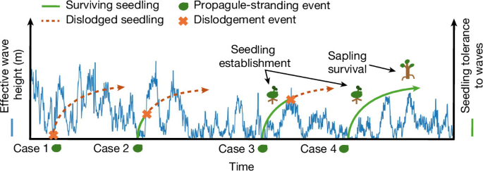
Global Wave Climate Analysis of Mangrove Establishment and Habitat Suitability

Study design and site selection

Global mangrove and non-mangrove sites

This study analyzed 20 years of wave data at 400 globally distributed coastal sites using a 3-hour temporal resolution. Sites were selected across all continents containing mangroves—Africa, Asia, North America, Oceania and South America—and extended to the latitudinal boundaries of mangrove distributions. The dataset therefore covered a broad range of mangrove genera and climates.

The selected dataset included 200 sites with mangroves on the open coast and 200 sites without mangroves. Mangrove presence and absence were identified using distribution data from Global Mangrove Watch⁵⁰ and cross-referenced with Google Earth satellite imagery from 2025.

Sites with mangroves were included only when the mangroves appeared to be exposed to waves, based on visual inspection of satellite imagery. Back-barrier mangroves protected from offshore waves by a dune or reef were excluded. Sites protected by a barrier reef or offshore island were permitted when the barrier was more than approximately 20 km away, corresponding to the resolution of the wave-model mesh. This included, for example, sites near the Great Barrier Reef. Embayed sites were also permitted when the bay or gulf was wider than 20 km.

To reduce the influence of climate on mangrove distribution, non-mangrove sites were selected within marine ecoregions that contain mangroves. These sites were identified using 2025 Google Earth imagery in coastal environments that appeared to consist of sand or mud. Rocky headlands were excluded. Sites with visible development that could prevent mangrove growth, including hardened shorelines and seawalls, were not selected.

Wave data and coastal measurements

Wave conditions were obtained from the Global Ocean Waves Reanalysis⁴⁸ of the EU Copernicus Marine Service Information: https://doi.org/10.48670/moi-00022. The dataset provides global spectral wave data at a spatial resolution of 0.2° × 0.2° and a 3-hour temporal resolution.

The product is based on MFWAM, a third-generation spectral wave model. It calculates the wave spectrum using ERA5 climatological winds⁵¹, GLORYS12V1 currents⁵² and ETOPO2 bathymetry⁵³. The analysis used 20 years of wave data, from 1 January 2003 through 1 January 2023.

Three spectral wave partitions were considered: the primary swell, secondary swell and wind components. The coastline bearing at each site was measured to the nearest 5° in QGIS using the 2025 Google Earth basemap.

Wave orbital velocity and hydrodynamic habitat thresholds

Significant wave height and wave direction were used to represent the magnitude of wave interaction at the shoreline. The physical mechanisms most likely to cause mangrove mortality through wave action are near-bed orbital flow velocity and erosion caused by bed shear stress¹⁹. For mangrove seedlings, whose diameters are D ≪ 1 m, inertial forces caused by near-bed flow acceleration can be considered negligible.

The drag force F_D caused by flow velocity u acting on a submerged structure is:

Here, C_D is the drag coefficient, A is the projected area and ρ is seawater density.

Mean bed shear stress is:

In this equation, f_w is the wave friction factor. Both mechanisms involved in mangrove seedling dislodgement—drag forces and erosion—are therefore driven largely by bed flow velocity.

The maximum horizontal component of wave-induced bed flow velocity is:

Here, H is wave height, ω is wave angular frequency, T is wave period, h is water depth and k is wavenumber. The angular frequency and wavenumber are defined as \(\omega \equiv \frac{2\pi }{T}\) and \(k\equiv \frac{2\pi }{\lambda }\), respectively.

In shallow water, where wavelength is approximated by \(\lambda \approx T\sqrt{{gh}}\) and \(\sinh (kh)\approx kh\), the equation becomes:

Here, g is gravitational acceleration. This approximation supports the use of significant wave height, H_s, as the offshore wave property most suitable for representing mangrove seedling establishment thresholds.

Effective wave height and wave refraction

When an offshore wave approaches the coast, refraction changes its height. The refracted wave height, H_r, is:

Here, H₀ is incident wave height and K_r is the refraction coefficient:

The angle \({\theta }_{0,\perp }\) is the angle between the offshore wave and the shore-normal direction. The angle \({\theta }_{\perp }\) is the corresponding angle for the refracted wave.

The analysis assumed that waves at the shoreline travel perpendicular to the coast. Under this assumption, nearshore wave height is:

To capture the spectral component with the greatest potential impact on each coastline at every 3-hour timestep, effective wave height (EWH) was defined as:

The EWH calculation used offshore significant wave height, H_s, and the mean wave direction relative to the beach normal, \({\theta }_{\perp }\), for each spectral partition. EWH represents the wave-spectrum component expected to have the greatest effect at a site at time t.

The maximum value among the swell partitions was used instead of bulk statistics for the complete spectrum. This approach captures conditions in which the mean spectral direction would produce a low EWH value, such as \({\theta }_{\perp ,m}\approx \pm {90}^{^\circ }\), even though an individual swell partition approaches the shoreline from a more influential direction, such as \({\theta }_{m}\approx {0}^{^\circ }\). Extended Data Fig. 1 illustrates the EWH calculation.

This parameter accounts for non-locally generated swell and varies through time, allowing the analysis to identify low-energy windows that may be important for mangrove establishment.

Twenty years of spectral wave data were extracted for each of the 400 analysis sites from the nearest offshore non-null wave-model node⁴⁸. Nodes were classified as offshore when the bearing between the node and the analysis site approached the coast at an angle between −90° and 90° relative to the shore-normal direction. Three mangrove sites and three non-mangrove sites were removed because all surrounding offshore nodes were null. EWH was calculated at every site for each 3-hour timestep.

Predicting mangrove establishment

Seedling establishment windows

A deterministic model was developed using the training sites. Mangrove seedling establishment thresholds were calculated from wave data at sites with mangroves.

Potential establishment periods of up to one year were defined as D_s = {1 day, 2 days, 5 days, 10 days, 2 weeks, 4 weeks, 8 weeks, 12 weeks, …, 52 weeks}. The increasing durations represent the increasing tolerance of mangrove seedlings to disturbance as they grow³². Shorter durations were sampled more frequently to capture the rapid initial anchoring of seedlings²². Durations up to one year were included to account for site seasonality.

For each site, the minimum thresholds that produced a period of non-exceedance for the first critical duration of 1 day were determined for each month. These thresholds, C_M,1d, were defined as:

Here, EWH_M(t) includes all EWH values for the specified month at the site. Each duration was then considered a candidate period for early propagule establishment.

For each set of co-originating durations \(D\in {D}_{{\rm{s}}}\), the maximum EWH value was determined. These periods represent windows during which hydrodynamic thresholds for seedlings of a given age should not be exceeded for establishment to succeed. The non-exceedance threshold for each duration D after the 1-day threshold C_M,1d was defined as C_M,D:

Because the initial thresholds were calculated from the beginning of each month, the method produced 12 sets of non-exceedance values per year at each site. Each set contained one threshold for every duration \(D\in {D}_{{\rm{s}}}\) and was treated as a candidate seedling establishment event.

Propagule availability can limit establishment in many environments¹⁵. However, global trends indicate that propagule abundance is typically lowest during winter⁵⁴, when wave energy is higher. This suggests that, globally, wave conditions during optimal establishment periods will generally coincide with propagule availability. Exceptions exist, and future site-specific studies should incorporate local propagule seasonality.

Establishment thresholds

The training sites included all sites except the site being assessed, consistent with the leave-one-out cross-validation method described in the Model performance section. Sites with and without mangroves had different distributions of non-exceedance values (Fig. 3a).

Anderson–Darling k-sample tests were used to compare these distributions for each duration. To ensure independence, the average non-exceedance value for each duration at each site was used, with n₁ = n₂ = 197. The results indicated that the null hypothesis—that mangrove and non-mangrove sites were drawn from the same distribution—could be rejected for all durations at the 2% significance level after Bonferroni correction for 18 tests. All tests produced P < 0.0011, while the corrected per-test significance level was α_corrected = 0.11%.

The 65th percentile of the threshold values at mangrove sites was selected as the upper establishment limit for seedlings of each age. This percentile was chosen by identifying the value that optimized the ratio of exceedance at non-mangrove sites to non-exceedance at mangrove sites, thereby providing the best combined specificity and sensitivity.

The resulting hydrodynamic habitat threshold, C_D, corresponded to each duration \(D\in {D}_{{\rm{s}}}\) (Fig. 3b). The thresholds were also recalculated separately for microtidal, mesotidal and macrotidal environments to evaluate the influence of tidal range. Tidal classifications were obtained from a dataset³⁰ based on the FES2014 global tide model³¹.

Comparison with previous empirical thresholds

The calculated thresholds were compared with previous empirical studies^27,32. The analysis produced an EWH threshold of 1.13 m for 12-month-old seedlings (Fig. 3; see the WOOs methods for the calculation).

Using a shallow-water breaking limit of \(\frac{H}{h}=0.78\) (ref. ⁵⁵), where H is wave height and h is water depth, this wave would break when water depth became shallower than 1.44 m. Beyond that point, linear wave equations would no longer apply.

In shallow water, the resulting near-bed wave orbital velocity was u = 1.46 m s⁻¹, calculated using equation (4). Previous work estimated that seedlings less than one year old may become vulnerable to uprooting at flow velocities of 1.2–1.5 m s⁻¹³², consistent with the present result.

Using a standard friction factor of f_w = 0.01 (ref. ⁵⁶) and a saltwater density of ρ = 1,025 kg m⁻³, the corresponding bed shear stress was τ_b = 10.88 N m⁻², calculated using equation (2). This value was within 2 standard deviations of the shear-stress limit previously imposed in models for seedlings of the same age²⁷.

Global mangrove-suitability prediction

The predictive approach was applied to 197 valid sites with mangroves and 197 valid sites without mangroves. A mangrove seedling was assumed to establish at a site in a particular year only when all hydrodynamic habitat thresholds were satisfied. A year was considered suitable when the following condition was met:

Previous studies^17,18 indicate that a single set of wave-related optimal establishment windows (WOOs) can be sufficient to initiate mangrove establishment. Mangrove stands may therefore remain present even when conditions become unsuitable outside the WOO. Accordingly, a site was considered suitable when the condition was met in any year included in the analysis.

The model produced a binary prediction of mangrove presence or absence. Results were first assessed across all sites and then for sites with Avicennia, Rhizophora or Sonneratia reported on the seaward fringe³³, allowing the response of different mangrove genera to hydrodynamic forcing to be examined.

Model performance and validation

Model performance was evaluated using accuracy, sensitivity and specificity.

True positives were sites predicted to contain mangroves that did contain mangroves. False positives were sites predicted to contain mangroves that did not. True negatives were sites predicted to lack mangroves that did not contain mangroves. False negatives were sites predicted to lack mangroves that did contain mangroves.

Leave-one-out cross-validation

The model was validated using leave-one-out cross-validation (LOOCV)⁵⁷. This method assesses predictions at every site. For each site, all other sites were used to train the model, and the trained model was then used to predict mangrove presence or absence at the remaining site.

In this analysis, training involved calculating the 65th percentile of the EWH non-exceedance values at all other sites. This percentile served as the establishment threshold for predicting mangrove establishment at the site being assessed.

Statistical testing

Differences between the distributions of EWH non-exceedance values at mangrove and non-mangrove sites were assessed using the Anderson–Darling k-sample test. Results were corrected for multiple comparisons using the Bonferroni correction.

The Anderson–Darling k-sample test⁵⁸ is a non-parametric extension of the Anderson–Darling test⁵⁹. It evaluates the null hypothesis that two or more groups are drawn from the same underlying distribution. The test was selected because it does not require specification of the population distribution and is sensitive to differences across the full distribution.

To ensure independence, the mean non-exceedance value calculated across all sampled monthly starting points was used for each duration at each site. The test computes the statistic A², which can be compared with a critical value to determine whether the null hypothesis can be rejected at the relevant significance level.

When multiple statistical tests are conducted, the probability of a type I error occurring in at least one test is greater than the probability of an error in any individual test. The Bonferroni correction addresses this by defining the adjusted significance level as⁶⁰:

Here, m is the number of tests. Statistical significance was evaluated using the Bonferroni-adjusted level corresponding to a family-wise error rate of 2%. For this study, the resulting per-test significance level was α_corrected = 0.11%.

Coastal case studies

Two case-study coastlines containing both mangrove and non-mangrove areas were selected. The first was located in the Palk Strait of the Indian Ocean, between 9.599069° N, 78.911753° E and 9.238059° N, 79.286306° E. The second was located in the Gulf of Thailand in the Pacific Ocean, between 9.342269° N, 99.187294° E and 9.221632° N, 99.352620° E.

Equidistant points were created along each selected coastline at spacings of 0.05° and 0.1°. Shorelines at each point were visually classified as mangrove, non-mangrove or developed. Mangrove sites were classified using the method described in the Site selection section. Points with houses or other structures along the shoreline were classified as developed.

The model was then applied using the method described in the WOOs section and thresholds calculated from all 197 valid mangrove sites in the global analysis. Each point was classified as suitable or unsuitable for mangroves. The analysis was repeated after decreasing and increasing historical EWH values across a range of percentages.

Global sensitivity to changing wave climate

Sites correctly classified by the model as mangrove or non-mangrove were reassessed under altered wave conditions to evaluate sensitivity to changes in wave climate.

The 20 years of historical wave data used to predict current mangrove presence were multiplied by factors ranging from 55% to 145%, representing changes from −45% to +45%. Site suitability for mangroves was then recalculated using the modified wave data.

Reporting summary

Additional information about the research design is available in the Nature Portfolio Reporting Summary linked to this article.