


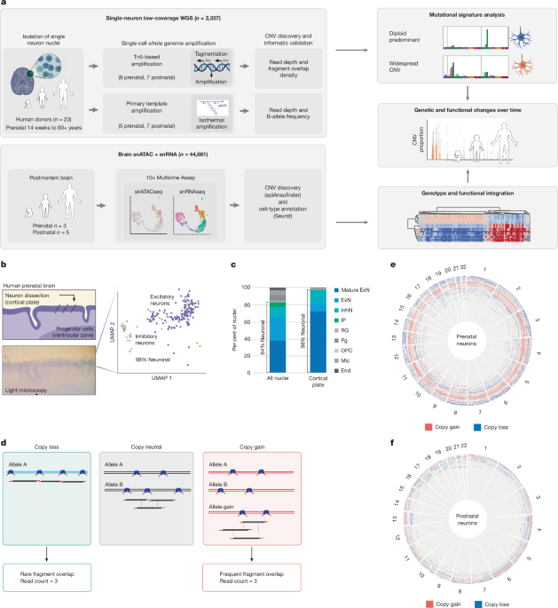
The study used human prenatal and postnatal brain tissue, neuronal nuclei, single-nucleus whole-genome sequencing, and single-cell multiomics to characterize somatic copy-number variants (CNVs) in individual brain cells. The researchers isolated nuclei, generated and quality-controlled sequencing libraries, called and validated CNVs, analysed copy-number signatures and genomic breakpoints, and linked CNV status to cell type and gene-expression programs associated with senescence, apoptosis, autophagy and other cell-elimination pathways.
Isolation of neuronal nuclei
Human prenatal brain tissue was obtained from the NIH NeuroBioBank. Frontoparietal-lobe tissue was cut into 40 μm sections with a cryostat. Researchers dissected the cortical plate with a microscalpel under a light microscope and dissociated it into nuclei by gentle Dounce homogenization in 1.5 ml of lysis buffer containing 10 mM Tris-HCl (pH 8.0), 250 mM sucrose, 25 mM KCl, 5 mM MgCl2, 0.1% Triton-X, 1× cOmplete Mini Protease and 1 mM DTT.
Nuclei were pelleted by centrifugation for 10 min at 900g. The supernatant was removed, and the nuclei were resuspended in sorting buffer consisting of 1× PBS (pH 7.4), 0.8% BSA and 0.1 μg ml−1 DAPI. Flow cytometry was used to isolate single nuclei based on forward scatter, side scatter and DAPI content. Postnatal brain nuclei were stained with both DAPI and Alexa Fluor 488-conjugated anti-NeuN at 1:1,000 for 1 h at 4 °C (Sigma Aldrich MAB377X), as previously described50.
Single-nuclei whole-genome library preparation
TbA has been used for single-cell whole-genome amplification (scWGA) in several contexts and under different names. Its core workflow comprises nucleosome depletion, Tn5 tagmentation with direct adapter addition, and library amplification.
Single nuclei were lysed in microwells containing 2 μl of lysis buffer with 20 mM NaCl, 20 mM Tris-HCl (pH 8.0), 0.15% Triton-X, 1 mM EDTA, 250 mM DTT and 0.05 μl thermolabile Proteinase K (NEB P8111S). Lysis was performed at 30 °C for 1 h, followed by proteinase inactivation at 55 °C for 10 min. Proteinase K digests nucleosomal histones, improving genome accessibility by removing chromatin structure.
Tn5 was loaded according to the manufacturer’s instructions (Diagenode C01070010-20). For each nucleus, 1 μl of Tn5 diluted 1,000-fold was used, and tagmentation was performed with the manufacturer’s buffers and instructions. Single-cell genome libraries were generated with 16 PCR cycles using NexteraXT v.2 indexes.
Rows containing 12 single cells were pooled for cleanup with the Zymo Clean and Concentrator Kit. Each row was eluted in 42 μl of Zymo elution buffer and then subjected to 0.8× AMPure XP size selection. Four rows, representing 48 cells, were pooled at equimolar concentration for sequencing on a NovaSeq 6000 (Novogene), targeting a library size of 0.5 Gb per single-cell library.
Illumina reads were aligned to the human reference genome containing the decoy sequence GRCh37d5 (hs37d5) with bwa-mem51. Duplicate reads were marked, and base-quality scores were recalibrated according to GATK best practices52.
Single-cell library quality assessment
To restrict analyses to high-quality single-cell genomes, cells with fewer than 10 million total covered bases were first removed. This value was taken from the “total” column in GATK DepthOfCoverage, which represents the summed per-base depth across all genomic positions.
The researchers then used a neural progenitor cell (NPC) line dataset for transfer learning to distinguish high- and poor-quality sequencing profiles. TbA libraries from NPC-line cells provided a quality benchmark. After 24 h of staurosporine treatment to induce apoptosis, the labelled dataset comprised recently viable, high-quality cells; Annexin V-positive apoptotic cells with intact nuclear envelopes; and propidium-iodide-positive cells with compromised nuclear integrity (Extended Data Fig. 1c).
The NPC line was differentiated as previously described53 from an induced pluripotent stem-cell (iPSC) line derived from well-characterized human fibroblasts54. NPC identity was confirmed on 21 March 2021 by immunohistochemistry using antibodies against PAX6 (BD Pharmingen 561462; 1:300) and Nestin (Millipore Sigma HPA026111; 1:500).
For computational classification, read counts in the NPC dataset were normalized with the read-depth normalization function of HiScanner34, using 500 kb bins to create a cell-by-bin matrix. Scanpy55 was used to scale read counts, standardize variance across cells and perform principal-component analysis. Cell-to-cell similarity was assessed with a neighbourhood graph constructed using scanpy.pp.neighbors.
Cells were clustered with the Leiden algorithm at a resolution of 0.2. After visual inspection and comparison of cluster-level read-count profiles with replication-timing tracks, library sizes and MAPD scores, the three Leiden clusters in the NPC dataset were classified as high quality, atypical and poor quality, respectively: QC Leiden 0, 1 and 2.
The researchers used scanpy.tl.ingest to project these labels and embeddings from the NPC dataset onto the human-brain single-cell TbA data using default parameters. Only cells labelled high quality (Leiden 0) with MAPD < 0.5 were retained. Samples were excluded if fewer than 65% of cells in a sample batch belonged to Leiden 0, because this suggested poor sample or batch quality. Batches yielding fewer than 25 cells after all cell-level filters were also excluded from downstream analyses.
Single-cell CNV calling
After cellular and sample-level filtering, CNVs were called on the single-cell genomes. For TbA data, calls were based on read depth and then validated using FOD, as described in the Supplementary Methods. For PTA data, CNV calling jointly used read depth and B-allele frequency (BAF).
TbA: CNV calling from read depth
HiScanner34 was run in rdr_only mode with parameters optimized for this analysis. The bin size was 500 kb of mappable positions, and hg19/GRCh37 was used as the reference genome. λ was set to 64, and ploidy restriction was enabled with max_wgd=1 and restrict_gamma=true. The multisample option was disabled (multisample=false) so that each cell was processed separately. HiScanner v.1.6.1 was installed through pip.
CNV candidates with P ≥ 0.05 or spanning less than 5 Mb were excluded. Candidates within the pseudoautosomal regions of chromosomes X and Y, as defined in the hg19/GRCh37 assembly, were also removed.
TbA: CNV validation with FOD
For each cell, a diploid FOD distribution was defined from the five longest segments predicted to have copy number 2, assuming that whole-genome doubling had not occurred. The mean and standard deviation of these segments were used to calculate FOD z-scores for each CNV candidate.
Calls were retained when the FOD z-score was greater than 1.96 for gains (CN > 2) or less than −1.96 for losses (CN < 2). Cells with a diploid mean FOD of zero were excluded. Calls that failed validation were reset to the diploid background value of 2.
PTA: CNV calling from read depth and BAF
Matched bulk whole-genome sequencing data were processed with the same alignment and preprocessing pipeline. For PTA data, HiScanner34 was run in BAF+RDR mode (rdr_only=false), using the matched bulk sample as the reference. The analysis used 500 kb mappable-position bins, λ = 64, max_wgd=1, an ADO threshold of 0.2 and restrict_gamma=true.
CNVs were reported as allelic copy numbers (CNA|CNB), with total copy number calculated as their sum. Post-processing filters were applied sequentially:
- Bins called as non-diploid in cells from three or more donors were treated as recurrent artefacts and reset to CN = 2.
- CNV segments shorter than 5 Mb were excluded.
- Putative homozygous deletions with the allelic pattern X∣0 were removed when inconsistent with the observed VAF (VAF > 0.1).
- Extreme copy-number states (CN > 4) were excluded.
- Gains (CN > 2) with VAFestimate < 0.2 were removed as likely artefacts.
Filtered regions were assigned the diploid background value of 2.
Copy-number signature analysis
Single-cell copy-number signature exposures were identified with SigProfilerAssignment v.0.1.4 and SigProfilerMatrixGenerator v.1.2.26 (refs. 56,57). The researchers first generated a 48-channel copy-number summary using COSMIC-defined channels.
Because the single-cell copy-number calls were not allele-specific, integer copy-number states were converted into pseudo-allele-specific states: 0 became 0|0, 1 became 1|0, 2 became 1|1, 3 became 2|1 and 4 became 3|1, continuing to a maximum copy number of 11, represented as 10|1. This conversion enabled the construction of 48-channel copy-number vectors compatible with existing signature-analysis frameworks.
The copy-number summaries were linearly decomposed into signature exposures with SigProfilerAssignment using default parameters and the COSMIC v.3.4 pan-cancer signature panel CN1–22, also called SigCN1–22 (ref. 36). Three cells with no callable CNV output, along with cells for which SigProfilerAssignment could not generate a valid decomposition, were excluded before signature clustering.
Each cell’s signature-exposure vector was normalized to sum to 1. Gaussian noise with σ = 10−4 was then added to resolve degeneracies in the sparse exposure space. For quality-filtered TbA cells (MAPD < 0.5), the researchers constructed a k-nearest-neighbour graph using k = 30 and cosine distance in Scanpy v.1.11.055. They generated a two-dimensional UMAP embedding and applied Leiden community detection at a resolution of 0.1.
This analysis identified four groups: cluster 0, predominantly diploid; cluster 1, predominantly gains; cluster 2, predominantly focal losses; and cluster 3, predominantly broad losses. PTA cells were mapped onto the TbA reference embedding with Scanpy’s ingest function, which transfers labels through k-nearest-neighbour mapping in the reference UMAP space.
To assess the decomposition, cosine similarity was calculated between each observed copy-number profile and the profile reconstructed from its assigned signature weights. Values close to 1 indicate that the signatures closely reproduce a cell’s copy-number landscape; lower values indicate poorer agreement with the reference panel. Cosine similarities were aggregated and compared between clusters as a measure of decomposition confidence.
Breakpoint distribution analysis
The researchers examined the relationship between CNV breakpoints and replication timing or DNA double-strand breaks (DSBs). For replication-timing analysis, they used the BG02ES human embryonic-stem-cell replication-timing track generated by ENCODE58,59 and downloaded from the UCSC Genome Browser60. The mean replication-timing signal was calculated for each 500 kb mappable bin and normalized from 0 to 1.
BLISS coordinates for DSBs were downloaded from FigShare (https://doi.org/10.6084/m9.figshare.18530531.v2)61. DSB BED files for each replicate were intersected with 500 kb genomic bins, and DSB signals were normalized to the maximum value in each track.
To create a background distribution for CNV-enrichment analyses, the researchers generated 10,000 random CNVs for every original CNV while matching its length distribution across autosomes (chromosomes 1–22). Pericentromeric and telomeric regions were excluded to reduce bias. Centromeric regions were defined by extending UCSC cytoband coordinates by ±5 Mb, while telomeric regions were defined as the first and last 5 Mb of each chromosome.
Replication-timing values were divided into deciles representing genomic quantiles. For each decile, the observed-to-expected (O/E) ratio was calculated by comparing observed CNV breakpoints—the start and end positions of each CNV—with the expected number from random simulations. Correlations between replication-timing O/E ratios for different CNV categories, including age groups and signature groups, were assessed with Pearson correlation tests.
CNV breakpoint distributions were also compared with BLISS data from six neural-cell preparations: two biological replicates each of human neuroepithelial stem cells, NPCs and postmitotic neurons (NEUs). BLISS read counts were summed into 500 kb bins and normalized to the maximum value in each track.
DSB hotspots were independently defined for each track as bins above the 99th percentile of normalized signal. A bin was classified as a hotspot if it exceeded this threshold in any of the six tracks. For each CNV, 10 length-matched random CNVs were generated by placing segments of the same length at uniformly sampled positions across the autosomes. Breakpoint positions were extracted from both the observed and simulated CNVs.
For each individual, O/E ratios were calculated as the number of breakpoints overlapping hotspot or non-hotspot bins divided by the mean count across the 10 simulated replicates. Neuroepithelial stem-cell replicates were excluded from the primary analysis because they showed a strong correlation with replication timing (Pearson r = 0.50–0.53, FDR-corrected P < 0.05), substantially higher than the correlations observed for NPCs (r = 0.17–0.23) and NEUs (r = 0.15–0.24). NPC and NEU tracks were therefore used for the aggregated hotspot analysis.
O/E ratios were capped at 4 for visualization. Statistical significance was assessed with paired t-tests comparing hotspot and non-hotspot O/E ratios for each individual (n = 15 pairs for gains and 15 pairs for losses). P values were adjusted for multiple testing with the Benjamini–Hochberg FDR procedure.
Breakpoints were also stratified by recurrence. A breakpoint was considered recurrent when the same genomic position appeared in more than one donor. Breakpoints detected in more than two donors were used for full-CNV recurrence analysis. A breakpoint was considered private when it was detected in exactly one cell from a single donor. Within-donor clonal breakpoints, shared by two or more cells from the same individual, were analysed separately. BLISS hotspot enrichment was performed independently for each recurrence class.
CNV gene-set enrichment analysis
To identify genomic hotspots and coldspots in diploid-predominant neurons, the researchers adapted an approach similar to that used in ref. 18. They defined 5 Mb genomic bins by aggregating the 500 kb coordinate set used for CNV calling. Small remaining segments at the ends of chromosomes were discarded.
Each 5 Mb bin received an empirical overlap count representing the number of observed CNVs overlapping it. The researchers then performed 10,000 permutations while preserving CNV sizes. Overlap counts for random CNVs were calculated in each permutation to generate a null distribution for every bin.
Bins were classified using unadjusted one-sided empirical P values. Upper-tail P < 0.05 defined hotspots, lower-tail P < 0.05 defined coldspots, and all other bins were classified as neutral.
Each bin was assessed for overlap with gene sets including housekeeping genes from Gene Ontology; loss-of-function-intolerant genes62 (pLI > 0.9); SFARI autism genes63; neurodevelopmental-disorder genes64; schizophrenia genes64; postsynaptic genes65; COSMIC cancer-driver genes66; and epilepsy genes identified through the OMIM67 symptom search for “epilepsy”. Hypergeometric tests were used to assess over-representation of each gene set in hotspots and coldspots compared with all genomic bins.
Single-nuclei multiomic ATAC/RNA library preparation
Nuclei were isolated without dissection as described above and permeabilized after flow cytometry according to the 10× Genomics protocol “Nuclei Isolation from Complex Tissues for Single Cell Multiome ATAC + Gene Expression Sequencing” (Demonstrated Protocol CG000375).
Chromium Next GEM Single Cell Multiome ATAC + Gene Expression libraries were prepared according to the manufacturer’s manual, with adaptations that also enabled detection of complementary DNA strands, or duplexes68. Duplex information was not used in this study.
Cell-type and CNV annotation of multiomic data
The multiomic dataset comprised snRNA-seq and snATAC-seq data from prenatal and postnatal brain samples generated with the 10× Genomics protocol. Data were processed with the 10× Genomics Cell Ranger ARC pipeline v.2.0.1 and then analysed with the Seurat v.5.0.169 and Signac v.1.12.070 R packages.
Quality control for snATAC-seq nuclei
Prenatal and postnatal nuclei were filtered using several metrics. Multiplets were identified in snATAC-seq data with AMULET and removed. Thresholds for other metrics were selected by visually inspecting rank plots for all samples.
A lower threshold of 1,000 was used for total RNA molecules, RNA features—the number of genes—and total ATAC fragments to remove empty background nuclei. No upper threshold was applied because multiplet removal had already been performed.
Nuclei were also removed when nucleosome-signal values were below 0.32 or above 1.59, or when TSS-enrichment values were below 1.75 or above 6.80. A minimum fraction of reads in peaks of 0.5 was applied.
Cell-type annotation from snRNA-seq
Each sample was mapped to a reference sample. Separate references were used for prenatal and postnatal samples because their cell-type compositions differed. H29180_F4 was used as the prenatal reference. The postnatal reference was a downsampled reference from a previously published dataset71.
The prenatal reference was manually annotated after unsupervised clustering of normalized, principal-component-analysis-transformed RNA counts. Clusters were assigned using known marker genes for different cell types, and a UMAP representation was generated. For the postnatal reference, the annotations reported in ref. 71 were used.
Other samples were treated as query datasets and projected onto the appropriate reference UMAP with Seurat’s MapQuery function. This transferred the manually annotated cell-type labels to all samples in the multiomic dataset.
CNV inference from snATAC-seq
CNVs were called with the R package epiAneufinder v.1.1.372, using 100 kb windows and a minimum of 20,000 fragments per sample. The minCNVsize parameter was set to 0, making one 100 kb bin the minimum callable CNV size.
After CNV calling, calls were combined across samples by taking the intersection of bins present in all samples. For each cell, the researchers calculated the percentage of these bins containing either a gain or a loss. Tukey’s rule was then used to identify outliers: cells with a percentage above the third quartile plus 1.5 times the interquartile range (Q3 + 1.5IQR) were classified as CNV neurons, while non-outliers were classified as non-CNV neurons.
DGM analysis
The snRNA-seq component of the multiome dataset was analysed separately for prenatal samples (n = 3: UMB4827, UMB1932 and 29180_F4) and postnatal samples (n = 5: APGEQ, UMB1790, UMB4643, UMB1278 and UMB1864) because of differences in cell-type composition.
For each developmental group, sample-specific Seurat objects were merged while retaining sample identifiers. Gene-expression values were log-normalized with a scale factor of 10,000.
Pathway activation was assessed with module scores based on gene sets from the Molecular Signatures Database73, including Gene Ontology Cellular Component terms and curated C2 gene sets. For C2, only gene sets matching “senescence”, “apoptosis”, “autophagy” or “caspase” were included; these were collectively termed cell-elimination C2 pathways.
Module scores were calculated with Seurat’s AddModuleScore function using default parameters. This function calculates the mean expression of each gene set in a cell and subtracts the aggregated expression of randomly selected control gene sets with similar average expression, helping to account for differences in gene-expression-program complexity.
Associations between module scores and CNV-neuron status were tested with stratified permutation testing. For each module, the researchers calculated the observed difference in mean module score between CNV and non-CNV cells, referred to as the absolute observed difference. CNV-neuron labels were then randomly shuffled 10,000 times within strata defined by sample and cell type.
P values were calculated as the proportion of permuted differences exceeding the observed absolute difference and were adjusted with Bonferroni correction. To reduce confounding from cell-type-specific expression, analyses were performed separately for excitatory neurons, inhibitory neurons, progenitors and other cell types, and separately for prenatal and postnatal samples.
Clustering CNV neurons by DGM and cell-death pathways
Distinct CNV-neuron subpopulations were identified by hierarchical clustering of normalized module scores from selected pathways. Rather than using every available pathway, the analysis focused on the 10 most differentially activated modules from Gene Ontology Cellular Component and cell-elimination C2 pathways, ranked by the absolute observed difference defined above.
The module-score matrix was normalized by subtracting the mean and dividing by the standard deviation across cells. Hierarchical clustering used average linkage and cosine distance. Visual inspection of the dendrogram and assessment of cluster stability indicated an optimal cluster number of 2.
Heatmaps were generated with the seaborn clustermap function, with rows clustered by gene set and columns clustered by cell. The visualization showed two main cell clusters with distinct pathway-activation patterns.
Cluster assignments were assessed through cluster sizes and enrichment for CNV neurons using Fisher’s exact test. Cluster 1 contained 1,667 cells and cluster 2 contained 2,487 cells. Associations between cluster membership and CNV-neuron status were summarized with odds ratios and 95% confidence intervals. Multiple testing was corrected with the Bonferroni procedure.
Ethics statement
Human materials were used in accordance with state and federal regulations, with approval from the Boston Children’s Hospital and Mass General Brigham Institutional Review Boards.
Postmortem human brain tissue was obtained from the NIH NeuroBioBank, including the University of Maryland Brain and Tissue Bank; the Autism BrainNet Collection; the University of Washington Birth Defects Research Laboratory (BDRL); and the Mayo Clinic Brain Bank. The contributing biobanks obtained informed consent for research from donors or their next of kin, as approved by their respective Institutional Review Boards.
The NPC line was derived from a previously described control iPSC line generated from commercially available human fibroblasts54.
Reporting summary
Additional information about the research design is available in the Nature Portfolio Reporting Summary linked to the article.
Source: www.nature.com