


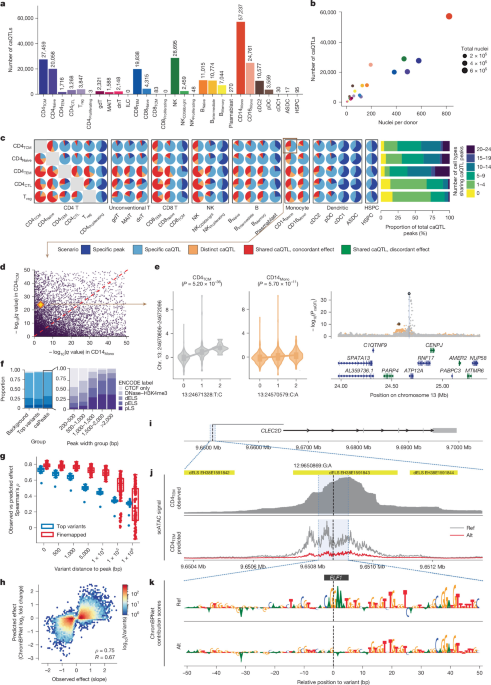
The study assembled and analyzed a large single-cell chromatin-accessibility dataset from human peripheral blood mononuclear cells (PBMCs) to map genetic variants that influence regulatory DNA activity across immune-cell types. Researchers processed samples from 1,042 participants in the TenK10K phase I cohort, generated single-cell ATAC-seq and multiome data, integrated these results with whole-genome sequencing, single-cell RNA sequencing, GWAS and eQTL data, and identified 243,225 chromatin-accessibility quantitative trait loci (caQTLs). The analyses also examined rare variants, cell-state-dependent effects, peak–gene links, gene-regulatory networks and potential drug targets.
Sample collection and library processing
To build a chromatin-accessibility atlas for human PBMCs, the researchers collected blood from 1,042 consenting participants in the TenK10K phase I cohort5. The cohort comprised 952 participants from the Tasmanian Ophthalmic Biobank (TOB), 64 from the BioHeart (BH) cohort55 and 26 from the Liquid Biopsy Biobank (LBIO). The 952 TOB participants were selected from 982 participants of European ancestry in OneK1K10, the TenK10K pilot cohort. TOB samples were processed in different batches from the scRNA-seq samples used by Cuomo et al.5.
BioHEART recruited participants between 29 March 2016 and 2 May 2023. Participants either attended for clinically indicated cardiovascular imaging or had acute ST-elevation myocardial infarction. LBIO was established to collect peripheral blood from people with advanced cancer receiving intravenous therapy; recruitment began in December 2019 and remains ongoing. No statistical method was used to predetermine the sample size, and the study involved neither randomization nor blinding.
Ethics oversight
The study followed all relevant ethical regulations and was overseen by Human Research Ethics Committees at the Royal Children’s Hospital, Northern Sydney Local Health District, St. Vincent’s Hospital and the University of Tasmania. Ethics approval was obtained for TOB (protocol 2020/ETH02479), BioHEART (2019/ETH08376) and LBIO (2019/ETH13113). All participants provided informed consent.
Single-cell ATAC-seq
The researchers processed all 952 TOB participants using the 10X Genomics Chromium Next GEM Single Cell ATAC kit v2, which provided the principal dataset for caQTL mapping. Cryopreserved PBMCs were thawed, washed, counted and pooled into 119 pools of eight participants, with equal numbers of live cells contributed by each donor. The team isolated and transposed nuclei, then ran each pool across two single-cell reactions targeting between 20,000 and 50,000 nuclei. The target for each library is listed in Supplementary Table 1.
In total, the researchers generated and sequenced 238 Illumina libraries at approximately 30,000 reads per nucleus. Sequencing used S4 flow-cell kits on the NovaSeq 6000.
Multiome sequencing
BioHEART and LBIO samples were processed with the 10X Genomics Chromium Next GEM Single Cell Multiome ATAC + Gene Expression kit v1. The 64-person BioHEART subcohort was divided into four pools of 16 participants. The 26-person LBIO subcohort was divided into four pools containing six or seven participants each.
As in the ATAC-only workflow, cryopreserved PBMCs were thawed, washed, counted and pooled with equal numbers of live cells per donor before nuclei were isolated and transposed. Each pooled suspension was run in a single reaction. ATAC and gene-expression libraries were generated from the same pool of pre-amplified transposed DNA and cDNA, then sequenced independently at approximately 30,000 reads per nucleus using S4 flow-cell kits on the NovaSeq 6000.
Whole-genome sequencing and genotyping
DNA for whole-genome sequencing (WGS) was extracted from blood with the Qiagen DNeasy Blood and Tissue Kit, and concentrations were measured with Qubit. Libraries were prepared with the KAPA PCR-free kit and sequenced on an Illumina NovaSeq 6000 at 30× coverage. Further quality-control and processing details were provided by Cuomo et al.5.
Genotype-array data for all 952 TOB participants were obtained from Yazar et al.10 and used only for demultiplexing. Twenty TOB participants lacked WGS data and were therefore excluded from caQTL mapping.
For common-variant caQTL mapping, the researchers selected common SNPs and indels with a minor allele frequency (MAF) of at least 5%. Variants with a minor allele count below 20 or a missing-genotype rate above 15% were excluded. Rare variants with MAF below 5% were extracted for rare-variant caQTL analysis. Genotype-array data generated with the Illumina Infinium Global Screening Array in OneK1K10 were also used for demultiplexing.
Quality control and preprocessing
Read alignment with Cell Ranger ATAC
Cell Ranger ATAC v2.2.0 was used to align reads to the GRCh38 v1.2.0 reference genome. The --force-cells parameter was set to 20,000, 40,000 or 50,000, depending on the targeted capture number for each library. This produced 9,457,411 nuclei in total (Supplementary Table 1).
For comparison, Cell Ranger ATAC v2.1.0, which lacked the --force-cells function and relied on automatic cell calling, produced 5,639,779 nuclei (Supplementary Table 2). Initial peaks were called with the built-in MACS2 method56. Cell Ranger ARC was used to process the BioHEART and LBIO multiome libraries, producing 105,887 nuclei.
Demultiplexing and doublet detection
Vireo, implemented through Demuxafy v2.1.057, was used to assign nuclei to donors and identify doublets. Because --force-cells was used during Cell Ranger processing, many low-quality nuclei were classified as unassigned during demultiplexing and removed; this affected 1,155,771 nuclei.
In the TOB cohort, 3,644,297 doublets were detected. The average doublet rate across the 238 libraries was 37.0%, compared with 32.7% when the force-cell setting was not used (Supplementary Table 3 and Supplementary Fig. 30). The researchers noted substantial differences in quality-control metrics between the two Cell Ranger versions, but said these were direct and expected consequences of the force-cell setting rather than inconsistencies in the underlying data. Both pipelines converged on essentially the same high-quality nuclei after standard quality control, and all downstream analyses used that filtered set.
Two donors, representing 10,003 nuclei, could not be matched to any donor genotype. After demultiplexing, 4,586,910 singlets from 950 donors remained.
For the BioHEART and LBIO multiome data, demultiplexing of the ATAC layer retained 41,248 singlets from 48 BioHEART donors and 15,303 singlets from 12 LBIO donors. One BioHEART library and two LBIO libraries were removed because of poor sequencing quality and demultiplexing performance. The gene-expression layer also had low data quality: only 11.9% of nuclei could be assigned reliably to a donor. Consequently, only the ATAC-layer results were used in downstream analyses.
Quality-control thresholds
Nuclei were excluded if they did not meet the following thresholds: more than 5,000 and fewer than 100,000 peak counts, more than 40% of reads overlapping peaks, a blacklist ratio below 0.01, a nucleosome signal below 4 and a TSS-enrichment score above 4.
Seven libraries containing fewer than 300 nuclei after quality control were excluded, resulting in the loss of one pool and eight donors. After matching against WGS data, a further 20 unmatched donors were removed. Seven libraries—S0268_2, S0301_1, S0302_1, S0303_1, S0304_1, S0304_2 and S0331_1—were removed after all quality-control steps.
The final dataset contained 3,472,552 nuclei from 922 TOB donors across 231 libraries (Supplementary Fig. 1). On average, each donor contributed 3,766 nuclei from scATAC-seq and 2,825 cells from matched scRNA-seq data.
Cell-type annotation by label transfer
To obtain detailed PBMC cell-type annotations, the researchers used a two-step strategy. First, they curated a multiome bridging dataset combining eight multiome datasets and 99,507 nuclei: six publicly available 10X datasets, the BioHeart dataset and the LBIO dataset. The datasets were merged into a shared peak space using the Reduce method, which combines intersecting peaks.
The bridging dataset was annotated by label transfer from a CITE-seq reference containing 120,678 cells, provided by Hao et al.58. Nuclei with a maximum prediction score below 0.3 were removed. The remaining dataset contained 95,348 nuclei representing 31 cell types, excluding three non-PBMC types (Supplementary Figs. 31 and 32).
After assigning labels to the bridging multiome dataset, the researchers built anchors for each ATAC library against the ATAC layer of the bridging dataset and transferred cell-type labels. Nuclei counts by cell type and library are reported in Supplementary Table 4, while donor-level counts for TOB, BioHeart and LBIO are reported in Supplementary Tables 5 and 6. Boxplots and principal-component-analysis plots were used to identify extreme donor-level outliers (Supplementary Figs. 33 and 34). The two technical replicates from each pool also showed reasonably high concordance (Supplementary Fig. 35).
The annotation strategy was designed to balance annotation accuracy with caQTL discovery power. After quality control, each donor contributed approximately 2,825 nuclei. Rare subtypes representing less than approximately 0.1% of cells could not be annotated reliably because many would contribute fewer than three nuclei per donor on average. The pooled design, with eight donors per library, also placed a practical limit on nuclei recovery.
Because caQTL power increases with the number of nuclei per donor and cell type, many fine-grained subtypes did not have enough representation for meaningful mapping. To test whether the annotation threshold affected the results, the researchers repeated chromosome 1 caQTL analysis for CD14Mono, NK, naive B and Treg cells using prediction-score thresholds of 0.3, 0.5, 0.7 and 0.9. Effect estimates were highly concordant with those from the original analysis, with Pearson’s R at least 0.88 in every condition (Supplementary Table 18 and Supplementary Fig. 36).
Differences from the identity line appeared mainly at the most stringent threshold of 0.9, which caused severe data loss in low-abundance populations. For example, that threshold left approximately four Treg nuclei per donor, which was not analytically viable. The researchers therefore used the highest-scoring assignment without an additional cutoff and selected 28 cell types as a balance between annotation fidelity and statistical power.
Verification of cell-type annotations with imputed scRNA-seq data
After assigning cell-type labels, the researchers examined canonical gene markers. They used the gene-activity scores generated during annotation and visualized markers from the Seurat58,59/Azimuth reference for CD14 monocytes and cDC1 cells. The corresponding populations showed enriched scores for their canonical markers (Supplementary Fig. 32). Marker activity for all 26 cell types in the main scATAC-seq dataset was also visualized (Supplementary Fig. 37).
Peak calling within each cell type
For each cell type, peaks were recalled from raw fragment files using MACS356, integrated into SnapATAC2 (ref. 60). The number of peaks ranged from 427 in CD8+ proliferating cells to 269,371 in CD16Mono cells, with a median of 170,292 (Fig. 1e).
Peaks were merged with the Reduce function in Signac61 to create a consensus list. The merged object contained 440,996 unique peaks, with minimum, median and maximum widths of 201 bp, 499 bp and 5,545 bp, respectively.
The peak regions were compared with ENCODE v4, which contains 2,348,854 peaks; a whole-body scATAC-seq atlas containing 1,154,611 peaks63; and the 10X 10k PBMC ATAC v2 Chromium Controller dataset, containing 164,487 peaks and 10,246 nuclei. After matching, 44,015 peaks, or 9.98%, did not overlap any of the three datasets (Supplementary Table 7).
The researchers suggested that the novel peaks probably resulted from the larger sample size, which provided greater power to detect regions with low accessibility. Donor-level sparsity was consistently higher for novel than known peaks (Supplementary Fig. 12), and ChromBPNet also showed lower prediction accuracy for novel peaks (Supplementary Fig. 11).
The peak list was annotated using functional categories based on overlaps with pre-annotated regions. In total, 437,561 peaks were assigned to 65 functional categories. A peak could belong to multiple categories, and category proportions were calculated from all matched peak–category pairs. The five main ENCODE v3 categories were promoter-like signature (pLS), proximal enhancer-like signature (pELS), distal enhancer-like signature (dELS), DNase–H3K4me3 and CTCF only64.
Dimensional reduction and visualization
EpiScanpy65 was used to create a reduced-dimensionality representation of the scATAC-seq data. Quality-controlled data were combined into one AnnData object without removing the 20 donors lacking matched WGS data, producing 3,546,117 nuclei and 440,996 peaks.
The data were binarized, and the 50,000 most variable peaks were selected using EpiScanpy’s built-in feature-variability score. Counts were then normalized so that each cell’s total count equaled the median total count before normalization. PCA was performed with Scanpy66, and the resulting clustering pattern was as expected (Supplementary Fig. 38).
The scATAC-seq data were integrated with TenK10K scRNA-seq data by projecting both into a shared co-embedding space (Extended Data Fig. 2a). One cluster showed limited overlap between the two modalities, which the researchers attributed to differences in the proportion of monocytes between datasets because the blood samples were processed in different batches. A more detailed explanation is provided in supplementary note 1 of the TenK10K flagship paper5.
caQTL mapping
After nucleus- and sample-level quality control, the downstream analyses used 3,472,552 scATAC-seq nuclei from 922 individuals, 5,438,679 scRNA-seq cells from 1,925 individuals—including the 922 individuals with scATAC-seq data—and 95,728 multiome nuclei from 60 individuals independent of the other two cohorts. Together, the datasets contained approximately 9 million cells or nuclei (Extended Data Fig. 1b).
Cell-type-specific caQTL mapping
To identify genetic variants associated with differences in chromatin accessibility, the researchers tested SNPs and indels against accessibility levels in each of the 28 cell types. Peak counts were summed across nuclei from each donor to create a cell-type-specific pseudobulk matrix. This was done separately for each sequencing repeat.
GC-content bias was corrected with the withinLaneNormalization function in EDAseq67. Peaks with zero counts in more than 95% of donors were removed. Counts were converted to counts per million and normalized to z scores. The two repeats were merged by averaging z scores for overlapping peaks; unique peaks retained their original scores. Each peak was then re-standardized across all donors.
The standardized matrix was used to generate chromatin-accessibility principal components. Sensitivity analyses evaluated normalization methods, window sizes and the number of principal components (Supplementary Figs. 39–41). Although a 10-kb window produced more significant associations, it would have missed associations outside that interval and reduced the number of variants overlapping other QTL datasets. To maintain consistent SNP–peak pairs between caQTL discovery and colocalization, the researchers used a default window of ±1 Mb around each peak centre.
The association model included sex, age, genotype principal components and chromatin-accessibility principal components. The number of donors per cell type ranged from 120 to 922. CD8+ proliferating cells, represented by three donors, and innate lymphoid cells, represented by 19 donors, were not tested because of limited sample size.
The number of principal components was selected with the Elbow method in PCAForQTL68. Each peak was tested against SNPs within ±1 Mb of its centre. The number of variants tested per peak ranged from 293 to 30,942, with a median of 6,067. TensorQTL69 performed 10,000 permutations per peak and corrected P values using a beta-approximation strategy. Peak-level correction was then applied within each chromosome. A caQTL was called at q < 0.05, producing 243,225 caQTLs. GPU acceleration was used to reduce the computational time required for the association tests.
Because each pool was measured twice, caQTL associations were also calculated separately for each repeated library. Significance levels, measured as −log10(q), and effect sizes were largely consistent between runs, with Pearson’s correlation above 0.90 across cell types except for rare cell types with limited power (Supplementary Fig. 42).
Cell-type specificity of caQTL effects
The researchers evaluated cell-type specificity using the approach described by Cuomo et al.5 (Fig. 1c, Extended Data Fig. 3 and Supplementary Fig. 5). For a caQTL identified at q < 5% in cell type A, they compared the associated caPeak with cell type B and defined five possible scenarios:
-
Scenario 1, specific caPeak: the caPeak was not sufficiently accessible—defined as accessible in fewer than 1% of nuclei—in cell type B.
-
Scenario 2, specific caQTL: the caPeak was sufficiently accessible in cell type B, but no caQTL was identified there.
-
Scenario 3, distinct caQTL: different caQTL variants in low linkage disequilibrium, with r2 < 0.5, were identified for the same caPeak in cell types A and B.
-
Scenario 4, shared caQTL with concordant effect: the same variant, or variants in high linkage disequilibrium with r2 ≥ 0.5, was identified for the same caPeak in both cell types, with the minor allele having the same directional effect on accessibility.
-
Scenario 5, shared caQTL with discordant effect: the same variant, or variants in high linkage disequilibrium with r2 ≥ 0.5, was identified in both cell types, but the minor allele had opposite directional effects.
Functional annotation of caQTLs
The 243,225 caQTLs spanned 100,483 peaks and 158,251 unique top variants. As with the chromatin peaks, the researchers overlapped caPeaks and the top variant for each peak with the five ENCODE v3 candidate cis-regulatory element categories (Fig. 1f). CaPeaks were further divided into five subgroups according to peak width.
Fine-mapping causal caQTL variants with SuSiE
SuSiE28 was used to fine-map variants for all caPeaks. For each peak, the analysis included variants within a 1-Mb cis window. Variant correlation matrices were calculated with PLINK v1.970, while z scores came from TensorQTL summary statistics. The sample size, N, was defined as the number of donors containing the relevant cell type.
These summary statistics were supplied to the susie_rss function with L = 10. The analysis produced credible sets for each peak and marginal posterior inclusion probabilities (PIPs) for individual variants.
Replication in published and in-house datasets
To assess replication, the researchers collected caQTL results from two published studies20,21. Because those studies used different cell-type annotations, a caQTL was considered replicated if a significant signal overlapped in the closest corresponding cell type. Directional replication was also assessed for Benaglio et al.21.
Because peak definitions differed among studies, replication was defined by overlap between peak regions, which could inflate concordance estimates. Fewer than 10% of the caQTLs replicated in previous studies, as expected given the lower statistical power of those earlier cohorts.
The researchers also mapped caQTLs in a combined multiome dataset of 60 quality-controlled donors from BioHeart and LBIO, using the same cell-type annotation, pseudobulk and association procedures as in the main TOB analysis.
For an allele-specific analysis, per-donor scATAC reads from 890 donors were realigned with STAR v2.7.11b in WASP mode71, retaining reads tagged vW:i:1 to correct allelic mapping bias. Heterozygous sites were obtained from phased, imputed OneK1K SNP-array genotypes, using MAF ≥ 0.05, imputation R2 ≥ 0.3 and biallelic SNPs only.
Reference and alternate snATAC counts at heterozygous sites were quantified with GATK ASEReadCounter v4.6.2 in per-donor, per-cell-type pseudobulk BAM files. Haplotype counts were resolved for each individual using phased genotypes and summed across each peak interval.
The researchers developed an optimized Python reimplementation of the mixQTL ASC method29. It was run with per-peak haplotype counts within a 1-Mb cis window around each peak, using default mixQTL parameters. Lead caQTLs were compared between TensorQTL and mixQTL using sign concordance and Spearman and Pearson correlations for peak-internal lead caQTLs that were measurable by ASC.
A lead caQTL was considered ASC-measurable if it met the default mixQTL thresholds, namely asc_cut-off = 5 and n_cut-off = 15. This required at least 15 donors with at least five SNP-intersecting reads for each haplotype within the peak. Cell types with fewer than 30 such lead caQTLs were excluded from headline correlation and concordance analyses to ensure stable estimates.
Rare caQTL mapping with SAIGE-QTL
The effects of rare variants on single-cell chromatin accessibility were assessed with the set-based test in SAIGE-QTL. All SNPs and indels with MAF below 5% and missingness below 15% were included. For each peak, variants within ±100 kb of the peak centre were tested together. This window was selected because it produced the largest number of caQTLs in a chromosome 1 and CD4 naive-cell sensitivity analysis (Supplementary Fig. 13).
Both burden and sequence kernel association tests (SKAT) were performed. Peak-level P values were combined with the Cauchy method, following the SAIGE-QTL paper31. Multiple testing was controlled with q values, and results with a false discovery rate below 5% were considered significant.
To determine whether rare signals were driven by common variants in linkage disequilibrium, the researchers performed conditional analyses. For each peak, they conditioned on the common variant with the lowest P value within a 100-kb cis window, based on TensorQTL results. After stepwise conditioning, 53,195 significant rare caQTLs remained significant in the set-based test.
Regulatory-effect prediction with ChromBPNet
Processing single-cell ATAC-seq data
Sequencing depth was normalized and the 238 scATAC-seq libraries were aggregated. Fragments were pooled by predicted cell type to create pseudobulk fragment files. The fragments were randomly divided into two pseudo-replicates, and peaks were called with the ENCODE ATAC-seq pipeline v2.2.3 using default parameters (https://github.com/ENCODE-DCC/atac-seq-pipeline). The overlap between the two peak sets was used in downstream analyses.
ChromBPNet bias-model training
To select initial bias-model hyperparameters, the data were divided into training, validation and test sets. Chromosomes 8 and 20 were used for validation, while chromosomes 1, 3 and 6 were used for testing.
Bias models were trained in three cell types with different numbers of cells: CD14 monocytes (n = 767,874), NK cells (n = 432,705) and naive B cells (n = 152,441). Bias-threshold factors from 0.1 to 1 were tested in increments of 0.1. The best model for each cell type was selected using three criteria: a high Pearson correlation between predicted and observed non-peak counts; a low but greater-than −0.3 correlation between predicted and observed peak counts; and capture of only bias motifs, such as Tn5 or DNase-I motifs, rather than genuine transcription-factor motifs in transcription-factor-MODISCO-derived motifs.
The ChromBPNet bias-factorized model30 was then trained with the best-performing model from each cell type. The final bias model was selected based on the highest correlation between predicted and observed peak counts and the lowest correlation between predicted and observed non-peak counts, while ensuring that Tn5 bias was corrected.
The final model, trained in NK cells with a bias-threshold factor of 1, was evaluated with fivefold cross-validation. The chromosome-partitioning scheme used by ChromBPNet30 assigned each chromosome to a test set exactly once across the folds.
Cell-type-specific ChromBPNet models
ChromBPNet models were trained in 25 of the 28 cell types using fivefold cross-validation and the selected final bias model. Models were not trained for CD8+ proliferating cells, which had four cells; innate lymphoid cells, which had 33 cells; or CD4+ proliferating cells, which had 145 cells.
Variant-effect prediction
For every top SNP associated with a peak, the researchers generated a 2,114-bp region centred on the variant, corresponding to the ChromBPNet input length. Cell-type-specific variant scores were calculated as the log2 fold change in predicted total counts for the alternative allele relative to the reference allele.
The same procedure was applied to fine-mapped SNPs with high PIP scores in each peak. Prediction accuracy was compared across different PIP thresholds (Supplementary Fig. 10).
Transcription-factor motif matching
Motif matching used the JASPAR 2026 vertebrate database72. Contribution scores were calculated for each variant, and motif discovery was performed with Tangermeme v0.5.1. The best-matching transcription factor was assigned according to the most significant motif P value near the variant.
Colocalizing caQTLs and eQTLs to identify peak–gene links
Peak–gene links were identified by integrating eQTL and caQTL summary statistics with coloc36. All significant caPeaks were tested against genes within ±1 Mb of the peak centre. Indels were excluded so that the same SNP list could be used across colocalization analyses.
Coloc estimates the posterior probability of five models: PPH0, no association with either trait; PPH1, association with trait 1 but not trait 2; PPH2, association with trait 2 but not trait 1; PPH3, association with both traits through two independent SNPs; and PPH4, association with both traits through one shared SNP. Here, trait 1 was chromatin accessibility and trait 2 was gene expression.
Colocalization indicates that a peak and gene may share a genetic signal, but it does not necessarily establish effect direction or size. To provide additional causal-inference support, the researchers used the Mendelian-randomization framework in OmicsSMR73.
CaQTL and eQTL summary statistics were converted to MatrixEQTL format and used to generate BESD files for SMR analysis. Only peaks with a nominal P < 5 × 10⁻⁸ were tested. This threshold was more stringent than q < 0.05, so OmicsSMR tested substantially fewer pairs than coloc. In CD14Mono, coloc tested 740,024 pairs, whereas OmicsSMR tested 191,423. After accounting for overlap, 190,494 pairs remained, meaning that OmicsSMR pairs represented 99.51% of the overlapping coloc set. Comparisons between methods were restricted to overlapping pairs.
Colocalization of caQTLs, eQTLs and GWAS associations
To investigate genetic mechanisms underlying GWAS associations, the researchers performed coloc analyses between caQTLs and GWAS results for 16 complex diseases, 25 blood serum markers and 19 blood-count traits. These traits matched those examined by Margoliash et al.74. EQTL–GWAS coloc results were obtained from Cuomo et al.5.
For additional comparison, bulk eQTL summary statistics were obtained from eQTLGen9, which included 31,684 participants, and GTEx v10 whole-body tissues, which included between 70 and 816 participants. The same colocalization analyses were performed with these datasets. SMR analyses were also run for eQTL–GWAS and caQTL–GWAS associations. For eQTL–GWAS SMR, genes with a top eQTL nominal P < 5 × 10⁻⁸ were tested.
GWAS loci were selected by clumping each GWAS at P < 5 × 10⁻⁸, linkage disequilibrium r2 < 0.01 and a ±1-Mb window. Raw eQTL and caQTL summary statistics and coloc and SMR results were then examined. For each locus, the researchers compiled genes and peaks with significant QTL associations at nominal P < 5 × 10⁻⁸.
A GWAS locus was considered colocalized with an eQTL or caQTL if at least one gene or peak met one of the following criteria: PPH4 > 0.8 in coloc or PSMR < 5 × 10⁻⁸ in SMR. Results were aggregated across cell types to calculate the overall proportion of GWAS loci that colocalized (Fig. 3a,b).
Because conventional coloc assumes a single causal variant for each phenotype, the researchers also used coloc.susie41 to account for multiple causal variants. SuSiE fine-mapping was performed separately for each phenotype, and every pair of credible sets was evaluated with conventional coloc. If any pair had PPH4 > 0.8, the phenotypes were considered colocalized.
Multi-trait fine-mapping of putative causal variants
The researchers applied mvSuSiE42, a variable-selection method for multivariate linear regression, to identify variants that may simultaneously affect disease risk, gene expression and chromatin accessibility.
Genes that colocalized with GWAS associations at PPH4 > 0.8 were selected as focal genes. For each focal gene, caPeaks that colocalized with its eQTL signal at PPH4 > 0.8 and lay within ±1 Mb of the gene body were selected. Summary statistics from eQTL, caQTL and GWAS analyses were combined into a z-score matrix, with SNPs as rows and phenotypes as columns.
Canonical covariance matrices for the remaining phenotypes were constructed with mashr27, and the linkage disequilibrium matrix for SNPs in each focal region was generated with PLINK70. These matrices and the z-score matrix were supplied to mvSuSiE.
The model produced credible sets intended to contain at least one causal SNP, PIP scores representing the probability that each SNP was causal, and posterior estimates of SNP effects on each phenotype. The local false-sign rate was used as the phenotype-level significance measure, with a cutoff of 0.01. Overall, 1,085 credible sets affected at least one phenotype layer (Supplementary Table 15); the analysis focused on sets affecting disease risk, gene expression and chromatin accessibility simultaneously.
Genetic regulation of cell state
Pseudotime inference with Palantir
To model cell-state progression, the researchers used Palantir76 on 1,176,697 cells from 942 donors across the CD4 lineage. The analysis included CD4 naive, CD4TCM, CD4TEM, CD4+ proliferating, CD4CTL and Treg cells.
Palantir infers pseudotime by projecting cells into diffusion space, constructing a neighbourhood graph and estimating progression from a user-defined starting population. It also models lineage probabilities toward terminal states with a Markov-chain framework.
The researchers first performed PCA using 75 components, followed by Harmony77 batch correction with sequencing pool as the batch variable. A UMAP embedding was generated from the corrected components using a 30-nearest-neighbour graph. The embeddings were then used to calculate 100 diffusion components. Palantir was run with k = 50 nearest neighbours and 8,000 waypoints.
Testing cell-state-dependent caQTL effects with CASTIE
Cell-specific pseudotime estimates from Palantir were analyzed with CASTIE43 within the SAIGE-QTL framework31 v0.2.5.1. CASTIE is designed to model heterogeneous genetic effects across cellular contexts directly from single-cell data without pseudobulk aggregation.
To reduce computational costs, the analysis included 493,520 cells from 386 donors. A null Poisson mixed model was first fitted for each gene across all cells. Pseudotime was included as the dynamic environmental covariate, while sex, age, genotype principal components and chromatin-accessibility principal components were included as static covariates.
Association tests were then performed for genetic markers with MAF > 0.01 and minor allele count > 5, processing 10,000 markers per chunk. Marker-level results were combined into gene-level P values with the ACAT test78.
For visualization, cells were divided into early, middle and late pseudotime groups spanning 0–0.33, 0.33–0.66 and 0.66–1.00, respectively.
Cell-function scores in CD4+ cells
Cell-function scores were calculated as cell states with scDeepID, a multitask transformer that uses biological pathway databases as prior knowledge. The model was trained on 2,390,948 CD4+ cells from TenK10K phase I scRNA-seq data, including CD4+ naive, CD4TCM, CD4TEM, CD4CTL, Treg and CD4+ proliferating cells.
The model used expression features from 4,000 highly variable genes selected with Scanpy’s highly_variable_genes function using n_top_genes = 4000, min_mean = 0.0123, max_mean = 3 and min_disp = 0.5. The human Reactome database provided pathway guidance, restricted to the 200 most informative pathways based on the presence of pathway genes among the highly variable genes.
The researchers extracted an attention-based latent space for UMAP visualization and cell-function scores. Each score was transformed to approximate a normal distribution with zero mean and unit variance.
Gene-regulatory-network inference with multiome data
Cell-type-specific GRNs with GLUE
GLUE47 was used to infer gene-regulatory networks in a cell-type-specific manner. Cells from each major cell type were combined across scRNA-seq and scATAC-seq datasets to create integrated objects.
For scRNA-seq, counts were normalized to each cell’s total, log-transformed and used to select 6,000 highly variable genes per major cell type. Expression values were clipped at max_value = 10 and scaled to unit variance. PCA with 100 components was followed by Harmony in Scanpy to account for technical differences between sequencing libraries.
For scATAC-seq, GLUE’s latent semantic indexing method was used for dimensionality reduction. The resulting components were used to construct a nearest-neighbour graph and generate a UMAP embedding in Scanpy with default parameters.
The GLUE guidance graph incorporated genomic proximity and regulatory evidence from eQTL data. An ATAC peak was connected to a gene with a positive edge if it lay within 150 kb of the gene promoter. Additional edges were added for peak–gene pairs in which the peak overlapped a locus associated with gene expression through an eQTL. Self-loops were included to improve numerical stability.
GLUE integrated the multiomic data using this guidance graph and learned low-dimensional embeddings for each data modality. Cis-regulatory inference was then performed from the embeddings. GLUE regulatory scores were calculated as the cosine similarity between gene and peak embeddings, with higher scores indicating stronger putative regulatory interactions.
Peak–gene pairs were labelled as having support if at least one putative regulatory signal, such as an eQTL, colocalized with the pair. SCENIC45 was then used to construct GRNs for each major cell type from the inferred peak–gene interactions.
To strengthen GRN inference, the researchers incorporated causal-inference results from SMR linking eQTLs and caQTLs. High-confidence peak–gene pairs were selected using an SMR threshold of P < 5 × 10⁻⁸. These interactions were used to enrich the cis-regulatory relationships inferred by GLUE and served as input for SCENIC-based GRN construction in CD14Mono. The curated links were intended to help identify transcription-factor–target-gene relationships that might otherwise be missed.
Paired and unpaired multiome data
To evaluate the benefits of incorporating eQTL data and compare inferred cis-regulatory scores, the researchers used a 10k human PBMC dataset from 10X Genomics processed with Cell Ranger ARC 2.0.0. They also randomly sampled approximately 10,000 cells from the TOB multiome cohort. Both datasets underwent the same preprocessing workflow, and GTEx and cell-type-specific eQTLs were incorporated into GLUE training.
QTL-derived and multiome-derived peak–gene links
Complementary analyses in CD14 monocytes compared peak–gene links from caQTL–eQTL colocalization with links inferred from multiome data using GLUE. Concordance was assessed with Spearman correlation and by binning GLUE scores according to increasing colocalization evidence. The analysis was repeated after restricting the comparison to pairs with PPH4 > 0.8.
The two methods measure different properties. QTL analysis asks whether a shared genetic variant affects both chromatin accessibility and gene expression, whereas GLUE infers links from patterns of covariation across cells. The approaches were therefore expected to produce partially overlapping but non-identical link sets. GLUE analysis was limited to peak–gene pairs within 150 kb and to highly variable genes.
Benchmarking peak–gene and GRN methods
The performance of GLUE was compared with existing methods in two benchmarking analyses. First, peak–gene links from GLUE47 and pgBoost49 were evaluated using the same GWAS79,80, eQTL75,81 and CRISPR validation sets used by pgBoost. The CRISPR references included studies by Thakore et al., Fulco et al., Ulirsch et al., Wakabayashi et al., Huang et al., Fulco et al., Gasperini et al. and Schraivogel et al.82–90.
pgBoost is a method for estimating variant-to-gene regulatory strength. The framework was modified to evaluate peak–gene links. For each method and validation set, candidate links were ranked by linking score. At each unique score, the enrichment of predicted links among true evaluation links was calculated as:
\(\frac{\frac{|{\rm predicted\ links}\cap{\rm true\ links}|}{|{\rm true\ links}|}}{\frac{|{\rm predicted\ links}|}{|{\rm candidate\ links}|}}\)
Candidate links were defined as all peak–gene pairs involving a gene scored by every method, with peak-to-TSS distances below 1 Mb and above 1 kb. For CRISPR analyses, candidate pairs were further restricted to those experimentally tested by CRISPR.
For each validation set, the maximum recall achieved by all methods was defined as R ≤ 1. Average enrichment across recall values was calculated as:
\(\frac{({\sum }_{i=1}^{{n}_{R}}{\mathrm{enrichment}}_{i}\times {(1-\mathrm{recall}}_{i}))}{{n}_{R}}\)
Here, \({n}_{R}\) denotes the number of true evaluation links corresponding to recall R. Standard errors for average enrichment and for differences between methods were estimated by bootstrapping genes over 1,000 iterations.
pgBoost was used as a reference for determining whether GLUE could achieve comparable results. In the 10X Genomics PBMC 10k multiome dataset, cells from four major cell types—CD14Mono, CD4TCM, CD4 naive and CD8 naive—were selected, with each type containing more than 1,000 cells.
GLUE, with and without TenK10K eQTL guidance, and pgBoost were applied separately to each cell type. Although GLUE normally uses the 6,000 most variable genes, the benchmark added 1,949 genes from CRISPR validation datasets, resulting in 7,233 genes. This accounts for the difference in peak–gene pair counts between the 10X benchmark and TenK10K discovery analyses. Performance was assessed by testing whether predicted pairs received higher scores when they belonged to the validation sets (Fig. 5a and Extended Data Fig. 9).
Second, GRN inference was benchmarked against CellOracle91 and SCENIC+46, two methods that integrate single-cell multiome data to infer GRNs. GLUE, with and without TenK10K eQTL and caQTL enhancement, and both comparison methods were applied to the 10X Genomics PBMC dataset to generate transcription-factor–target-gene pairs.
Three validation sets were assembled from transcription-factor knockout expression changes92, chromatin immunoprecipitation followed by sequencing data93–95 and functional protein–protein interactions96. Following established benchmarking practice97, early precision recall (EPR) was used. Early precision is the proportion of true-positive edges among the top k predicted edges. EPR is this value divided by the expected early precision of a random predictor, accounting for differences in network size and density. Error bars represent 95% confidence intervals, calculated as 1.96 times the standard error from five independent runs with different random seeds.
Drug-enrichment analysis
To determine whether single-cell caQTL data could help identify drug targets, the researchers analyzed target–indication pairs using the Open Targets Platform98 (OTP) v25.12, following an approach analogous to Henry et al.99.
Peak-to-trait SMR results were first used to shortlist peaks with putative causal effects on selected disease traits. These results were integrated with peak–gene SMR results to nominate candidate effector genes for each trait. Effector gene–trait pairs were then intersected with target–indication pairs in OTP. For drugs whose mechanisms of action matched the relevant target–indication pair, the highest clinical-development phase was recorded.
Pairs were stratified according to the highest clinical phase reached: phases I, II and III; combined categories I+, II+ and III+; and approved. For each category, a 2 × 2 contingency table counted target–indication pairs supported or not supported by caQTL-derived effector genes.
The researchers identified two important limitations. First, few target–indication pairs were supported by both caQTL evidence and clinical validation, so estimated odds ratios should be interpreted cautiously. Second, the analysis treated the absence of a caQTL- or eQTL-derived effector gene nomination as a negative result, even though this may reflect incomplete data rather than a true biological negative. Some apparently unsupported pairs could prove relevant as QTL mapping power improves or additional traits are incorporated. The enrichment results should therefore be regarded as a lower-bound estimate of concordance between QTL-nominated targets and established drug mechanisms.
Reporting summary
Additional information about the research design is available in the Nature Portfolio Reporting Summary linked to the article.
Source: www.nature.com