


Data Sources for Antarctic Ice Mass and Precipitation Variability
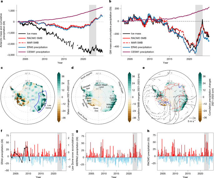
Antarctic ice-mass variability from 2003 to 2024 was quantified using GRACE and GRACE-FO satellite gravimetry data50. Surface mass balance (SMB)—calculated as precipitation minus meltwater runoff, sublimation, evaporation and wind erosion—was obtained from RACMO2.4p1 (ref. 51) and MARv3.14 (refs. 52,53). These datasets were used to identify how precipitation variability contributed to observed changes in Antarctic ice mass.
Precipitation variability was evaluated using several independent datasets, including the ERA5 (ref. 54) and MERRA-2 (ref. 55) atmospheric reanalyses and RACMO2.4p1 regional climate-model precipitation. Agreement among these datasets was assessed to improve confidence in the results. The Law Dome ice-core snow-accumulation record49 provided an additional observational constraint.
Large-scale atmospheric circulation and moisture transport were examined primarily with ERA5 fields, including sea-surface temperature (SST), geopotential height at 300 hPa (Z300), evaporation and integrated vapour transport (IVT). Velocity potential was obtained from NCEP–NCAR Reanalysis 1. The Niño 3.4, Indian Ocean Dipole (IOD), Interdecadal Pacific Oscillation (IPO), zonal wave-3 and Southern Annular Mode (SAM)56 indices were used to investigate their relationships with tropical western Pacific (TWP) variability.
To estimate the recurrence of TWP warming events, we analysed ERA5 data for 1950–2025 and the CESM1 Large Ensemble57. The model data included an 1,800-year fully coupled pre-industrial control simulation and 40-member historical and RCP8.5 simulations. Two paleo-reanalysis products were also used to independently assess the long-term relationship between TWP warming, the East Antarctic (EA) circulation dipole and Queen Maud Land (QW) precipitation. EKF400v2 (ref. 58) provides monthly Z500, 2-m air temperature and precipitation fields from 1603 to 2003. LMR v.2.1 (ref. 59) provides annual last-millennium ensemble reanalysis fields of Z500, SST and precipitation. Because EKF400v2 does not include SST, its 2-m air temperature field was used as a proxy for SST variability. Unless otherwise stated, monthly anomalies were calculated by removing the climatological seasonal cycle.
Based on the spatial distribution of ice-mass and cumulative precipitation anomalies, QW was defined as the region between 70–145° E and 65–75° S. The TWP was represented by an ellipse rotated 15° clockwise and centred at 135° E, 5° S. Its semi-major and semi-minor axes were 35° and 15°, respectively, based on the observed relationship between EA precipitation and tropical SST variability. The EA dipole index was calculated as the difference between area-mean Z300 anomalies over the EA high-pressure centre (55°–70° S, 120°–160° E) and the low-pressure centre south of Australia (30°–50° S, 80°–150° E).
Statistical Significance Testing
The significance of correlations, regressions and trends was evaluated using a two-tailed Student’s t-test at the 95% confidence level. Effective sample sizes were adjusted to account for autocorrelation in the time series.
$${N}^{* }=N\frac{1-{r}_{1}{r}_{2}}{1+{r}_{1}{r}_{2}}$$
(1)
Here, N is the total number of samples, while r1 and r2 are the lag-1 autocorrelation coefficients of the two correlated time series. For spatial fields, false discovery rate correction was additionally applied to control for multiple testing60.
Maximum Covariance Analysis (MCA)
Maximum covariance analysis (MCA)61 is a multivariate method that applies singular value decomposition to the cross-covariance matrix of two fields. It identifies paired spatial patterns and time series that maximise their shared covariance. Each MCA mode is a linear combination of the original variables and represents a distinct coupled variability pattern.
The contribution of each mode was measured using the squared covariance fraction, which indicates the proportion of total squared covariance explained by that mode. Larger values identify the leading modes of coupled variability. In this study, MCA was applied to deseasonalized and detrended monthly anomalies of ERA5 Z300 south of 23° N and Antarctic precipitation for 1979–2024.
Wave-Activity Flux Diagnosis
Stationary Rossby-wave propagation was diagnosed using the Takaya and Nakamura62 wave-activity flux (WAF) formulation. Horizontal WAF vectors (W) were calculated from geopotential-height anomalies relative to the climatological mean flow:
$$\begin{array}{c}{{\bf{W}}}_{{\rm{h}}}=\frac{p\cos \phi }{2|{\bf{U}}|}\\ \left(\begin{array}{c}\frac{U}{{a}^{2}{\cos }^{2}\phi }\left[{\left(\frac{{\rm{\partial }}{\psi }^{{\prime} }}{{\rm{\partial }}\lambda }\right)}^{2}-{\psi }^{{\prime} }\frac{{{\rm{\partial }}}^{2}{\psi }^{{\prime} }}{{\rm{\partial }}{\lambda }^{2}}\right]+\frac{V}{{a}^{2}\cos \phi }\,\left[\frac{{\rm{\partial }}{\psi }^{{\prime} }}{{\rm{\partial }}\lambda }\frac{{\rm{\partial }}{\psi }^{{\prime} }}{{\rm{\partial }}\phi }-{\psi }^{{\prime} }\frac{{{\rm{\partial }}}^{2}{\psi }^{{\prime} }}{{\rm{\partial }}\lambda {\rm{\partial }}\phi }\right]\\ \frac{U}{{a}^{2}\cos \phi }\left[\frac{{\rm{\partial }}{\psi }^{{\prime} }}{{\rm{\partial }}\lambda }\frac{{\rm{\partial }}{\psi }^{{\prime} }}{{\rm{\partial }}\phi }-{\psi }^{{\prime} }\frac{{{\rm{\partial }}}^{2}{\psi }^{{\prime} }}{{\rm{\partial }}\lambda {\rm{\partial }}\phi }\right]+\frac{V}{{a}^{2}}\left[{\left(\frac{{\rm{\partial }}{\psi }^{{\prime} }}{{\rm{\partial }}\phi }\right)}^{2}-{\psi }^{{\prime} }\frac{{{\rm{\partial }}}^{2}{\psi }^{{\prime} }}{{\rm{\partial }}{\phi }^{2}}\right]\end{array}\right)\end{array}$$
(2)
In this equation, \({\psi }^{{\prime} }\) is the anomalous geostrophic streamfunction derived from geopotential height (Z), defined as \({\psi }^{{\prime} }=g{Z}^{{\prime} }/f\). Here, g is gravitational acceleration and f is the Coriolis parameter. The climatological horizontal wind vector is U = (U, V), with magnitude \(|{\bf{U}}|=\sqrt{{U}^{2}+{V}^{2}}\). Longitude and latitude are denoted by λ and φ, respectively. The Earth’s radius is represented by a, and p is the pressure level normalized by 1,000 hPa.
Atmospheric River Detection
Monthly atmospheric-river (AR) frequency anomalies were regressed against standardized MCA3 Z300 time series to examine the relationship between AR activity and the EA dipole circulation. Atmospheric rivers were detected using the Guan and Waliser63 algorithm, an updated and validated method suited to high-latitude regions such as Antarctica, where background atmospheric moisture is low.
The algorithm uses seasonally and geographically varying IVT thresholds rather than a single global threshold. This design improves the identification of poleward moisture intrusions relative to local climatological conditions. Detection was applied to 6-hourly IVT fields calculated from wind and specific humidity integrated between 1,000 and 300 hPa:
$$\text{IVT}\,=\,\frac{1}{g}\sqrt{{\left({\int }_{1,000}^{300}{uq}{\rm{d}}p\right)}^{2}+{\left({\int }_{1,000}^{300}{vq}{\rm{d}}p\right)}^{2}}$$
(3)
Here, g is gravitational acceleration, u and v are the zonal and meridional wind components, and q is specific humidity. AR identification required three criteria63: (1) the IVT magnitude had to exceed the 85th percentile of the local monthly IVT climatology or 100 kg m−1 s−1, whichever was greater; (2) the feature had to exceed 2,000 km in length and have a length-to-width ratio greater than 2; and (3) the mean IVT direction had to show directional coherence, excluding features without consistent poleward moisture transport.
Monthly AR frequency was calculated from daily occurrence counts, with daily counts derived from the 6-hourly detections. The Guan and Waliser63 algorithm effectively captures ARs over the Southern Ocean but may be less reliable after landfall34,37. It was selected because the analysis required one consistent detection method across the Southern Hemisphere rather than a region-specific algorithm.
Eddy Vorticity Budget Analysis
To identify the dynamical processes responsible for forming and maintaining the meridional circulation dipole between the southern Australian low and the EA high, we analysed the relative-vorticity budget following ref. 64. The relative-vorticity tendency at a given pressure level is expressed as ref. 65:
$$\frac{\partial \zeta }{\partial t}=-\nabla \cdot [(\zeta +f){\bf{u}}]-\omega \frac{\partial \zeta }{\partial p}+\hat{{\bf{k}}}\cdot \frac{\partial {\bf{u}}}{\partial p}\times \nabla \omega +F$$
(4)
In this equation, ζ is relative vorticity, f is the Coriolis parameter, u = (u, v) is the horizontal wind vector, ω is vertical velocity in pressure coordinates and F represents frictional forcing.
Standard scaling arguments65 show that vertical-advection and tilting terms are at least one order of magnitude smaller than horizontal vorticity-flux convergence. These smaller terms were therefore omitted. Each variable was separated into a seasonal-mean component, indicated by an overbar, and an anomaly, indicated by a prime. The anomalous-vorticity tendency equation becomes64:
$$\frac{\partial {\zeta }^{{\prime} }}{\partial t}=\mathop{\underbrace{[-(\bar{\zeta }+f)\nabla \cdot {{\bf{u}}}^{{\prime} }-{\zeta }^{{\prime} }\nabla \cdot \bar{{\bf{u}}}]}}\limits_{{\rm{stretching}}\,{\rm{term}}}+\mathop{\underbrace{[-\nabla \cdot ({\zeta }^{{\prime} }{{\bf{u}}}^{{\prime} })]}}\limits_{{\rm{eddy}}\,{\rm{term}}}+\mathop{\underbrace{[-{{\bf{u}}}^{{\prime} }\cdot \nabla (\bar{\zeta }+f)-\bar{{\bf{u}}}\cdot \nabla {\zeta }^{{\prime} }]}}\limits_{{\rm{wave}}\,{\rm{term}}}+\mathop{\underbrace{\{-\nabla \cdot [\bar{{\bf{u}}}(\bar{\zeta }+f)]\}}}\limits_{{\rm{climatological}}\,{\rm{term}}}+{F}^{{\prime} }$$
(5)
The stretching term represents vorticity generation by anomalous divergence. The eddy term describes anomalous-vorticity flux convergence and the dynamical feedback between transient eddies—defined here as periods shorter than 7 days—and the low-frequency circulation. The wave term represents advection of background vorticity by anomalous winds and advection of anomalous vorticity by the mean flow, processes associated with Rossby-wave propagation. The climatological term contains only mean-state quantities and represents stationary-wave forcing. Because it varies weakly over time, it was excluded from the temporal correlation analysis.
Atmospheric General Circulation Model Sensitivity Experiments
We conducted sensitivity experiments with two atmospheric general circulation models (AGCMs)66, ECHAM5 and CAM5, to quantify the influence of TWP SST anomalies on precipitation over EA. ECHAM5 was run at T42 spectral resolution, approximately 2.8° × 2.8°, with 19 vertical levels extending to 10 hPa. The model used a standard AMIP-style configuration.
A 40-year control simulation was performed using monthly climatological SST and sea-ice concentrations from ERA5 for 1979–2024. Greenhouse-gas concentrations and aerosol levels were fixed at year-2000 values to exclude transient anthropogenic forcing. Eight 40-year sensitivity experiments were then conducted by adding prescribed SST anomalies to the control climatology. Atmospheric responses were calculated as the difference between each sensitivity experiment and the control simulation.
Experiment 1 applied positive SST anomalies over the TWP, defined as a 15° clockwise-rotated ellipse centred at 135° E, 5° S, with semi-major and semi-minor axes of 35° and 15°. Experiment 2 combined TWP warming with La Niña-like cooling in the eastern Pacific and negative IOD-like cooling in the northwestern Indian Ocean. The eastern Pacific cooling region was an ellipse centred at 130° W, 0° N, with axes of 60° × 15°, while the IOD-like cooling region was centred at 65° E, 5° N, with axes of 30° × 15°.
Experiments 3 and 4 isolated the effects of eastern-Pacific La Niña-like cooling and northwestern Indian Ocean IOD-like cooling, respectively. Experiment 5 applied positive SST anomalies over the South Pacific Convergence Zone (SPCZ), represented by a 10° clockwise-rotated ellipse centred at 200° E, 25° S, with semi-major and semi-minor axes of 60° and 8°. Experiment 6 added the TWP anomaly to a uniform 0.5 K warming across the tropical band from 30° S to 30° N. Experiment 7 used the same background warming but increased the TWP anomaly by an additional 0.5 K. Experiment 8 repeated experiment 1 with CAM5 to test whether the results depended on the model used.
For experiments 1–6 and 8, SST anomalies increased from ±0.5 K at the boundaries to a maximum of ±1 K at the centre. In experiment 7, the TWP anomaly ranged from 1 K at the edge to 1.5 K at the centre.
The MCA3 SST anomaly pattern and the mean SST anomalies during 2021–2023 showed that La Niña-like cooling, negative IOD cooling and SPCZ warming occurred alongside prolonged TWP warming. When both cooling patterns were imposed with TWP warming in experiment 2, the Z300 response featured a more localized low-pressure anomaly over southern Australia and a stronger high-pressure anomaly north of the Ross Sea. EA precipitation increased by an amount comparable to that in experiment 1.
In contrast, experiments 3–5, which separately tested La Niña-like cooling, IOD-like cooling and SPCZ warming, did not reproduce a significant EA dipole or positive precipitation anomalies near QW. This indicates that these SST anomalies were not the primary forcings behind the observed response.
CESM1 projections indicate that tropical mean SSTs will continue to rise. Mean SST during 2021–2050 is approximately 0.5 K warmer than during 1991–2020 across most of the tropics. Under the uniform tropical warming imposed in experiment 6, the Z300, surface-temperature and precipitation responses over EA were weaker and less significant. The reduced response likely reflects a smaller relative SST gradient between the TWP and surrounding regions, which weakens the associated convective heating anomaly. Increasing the TWP warming magnitude in experiment 7 restored a pronounced EA response, demonstrating that EA circulation is more sensitive to localized TWP SST gradients than to broad, basin-wide tropical warming.
Experiment 8 used CAM5 at 1.9° × 2.5° horizontal resolution with 30 vertical levels. It reproduced the north–south circulation dipole and enhanced EA precipitation found in the ECHAM5 experiments (Extended Data Fig. 9), confirming that the results were robust across models.
Moisture-Source Tracing and Atmospheric Transport
Moisture sources and transport pathways were quantified using the isotope-enabled CESM1.2 (iCESM1.2), which employed a finite-volume dynamical core at 1.9° × 2.5° resolution. The water-tagging and circulation-nudging configuration enabled moisture-source attribution under observed atmospheric circulation and temperature conditions.
Monthly SST and sea-ice concentrations were prescribed from ERA5. The model atmosphere was nudged towards ERA5 using the NCAR DART framework. Horizontal winds, temperature throughout the atmospheric column and near-surface specific humidity were relaxed towards ERA5 values using a 6-hour timescale:
$$\frac{{\rm{d}}x}{{\rm{d}}t}={F}_{\text{model}}(x)+\alpha \frac{{x}_{\text{ERA}5}-x}{\tau }$$
(6)
Here, Fmodel represents internally generated model-physics and dynamical tendencies, τ is the 6-hour nudging timescale and α = 1 indicates full nudging. This approach constrained the large-scale circulation while allowing the hydrological cycle and isotopic fractionation to develop freely.
The moisture-tracing method followed the isotope-enabled Community Atmosphere Model framework. Each water tag was treated as an isotope tracer without isotopic fractionation. Convection, cloud microphysics, condensation, precipitation formation and re-evaporation were simulated for each tagged component in water vapour, cloud liquid, cloud ice and precipitation using the standard Community Atmosphere Model physics.
Fifty-four geographically defined surface regions were assigned separate moisture tags. Water vapour evaporated from each region was tracked through atmospheric transport and phase changes without affecting radiation or dynamics. Contributions from each source to QW precipitation were calculated for the climatological mean, the 2021–2023 precipitation anomaly and the 2011–2020 precipitation deficit. The analysis tracked only the immediate, direct moisture contribution to the most recent precipitation event.
Mechanism Linking TWP Warming to East Antarctic Precipitation
By combining satellite gravimetry, reanalysis datasets, moisture-tagging simulations, nudged-model experiments and AGCM sensitivity tests, we identified a mechanism linking TWP SST anomalies with persistent high-latitude circulation changes and enhanced precipitation over QW. This mechanism helps explain both the abrupt ice-mass gains during 2021–2023 and the prolonged ice-mass loss observed from 2011 to 2020.
Persistent TWP warming generates upper-tropospheric divergence and Rossby-wave activity. The resulting wave train propagates poleward and reaches high southern latitudes, where it establishes a meridional circulation dipole. A high-pressure anomaly forms over the EA coast and is dynamically strengthened by eddy–mean-flow feedbacks. This circulation favours blocking over EA, increases poleward moisture transport and enhances precipitation near QW.
The additional precipitation over QW is driven mainly by circulation-related moisture transport from subtropical source regions and by atmospheric-river extremes (Extended Data Fig. 5e,f), rather than by increased local evaporation.
Empirical Mode Decomposition
Long-term SST records extending over more than a century may contain nonlinear trends. To isolate oscillatory variability from these trends, we applied empirical mode decomposition (EMD)67. EMD is an adaptive, data-driven method that separates a signal into intrinsic mode functions (IMFs) across different timescales without requiring predefined basis functions.
Each IMF met two conditions: (1) the number of local extrema and zero crossings differed by no more than one across the record; and (2) the mean of the upper and lower envelopes formed from local maxima and minima was zero at every point. The original signal X(t) was represented as:
$$X(t)=\sum_{i=1}^{n}\mathrm{IMF}_{i}(t)+r(t)$$
(7)
The first IMFs describe higher-frequency variability, while later IMFs represent progressively longer-period oscillations. The residual r(t) represents the long-term background trend remaining after all IMFs have been extracted.
Decadal Recurrence of Multiyear TWP Warming Events
MCA results and modelling experiments indicate that TWP SST anomalies play an important role in regulating precipitation variability over EA. However, the contribution of this mechanism before the GRACE observational period remained uncertain. An earlier QW precipitation increase occurred during 2000–2002, before GRACE began, and displayed a teleconnection pattern similar to but weaker than the 2021–2023 event (Extended Data Figs. 2a,b and 10c,d).
In contrast, the decade-long precipitation deficit from 2011 to 2020 was associated with circulation and SST anomalies in the opposite phase (Extended Data Fig. 10a,b). These contrasting periods demonstrate that TWP SST variability can modulate QW precipitation on decadal timescales and may provide a useful indicator of large-scale climate conditions linked to Antarctic precipitation extremes.
Because step-like increases in cumulative TWP SST anomalies consistently coincided with prolonged QW precipitation extremes, we developed a cumulative SST criterion to identify multiyear TWP warming events. The threshold was based on the magnitude and duration of the observed 2000–2002 and 2021–2023 events.
An event was identified when the cumulative TWP SST anomaly index increased by at least 4 K within 36 months. The event began at the preceding cumulative minimum. Once the threshold was reached, the cumulative index was followed until it declined by 0.4 K from its subsequent maximum. The month of that maximum marked the end of the event.
This criterion was applied to ERA5 data for 1950–2025, the CESM1 pre-industrial control simulation and the CESM1 historical ensemble. Before event detection, the EMD residual was removed from each long-term time series. Removing this nonlinear background trend allowed events to be identified relative to the evolving SST baseline and prevented isolated TWP warming episodes from being confused with long-term background warming.
ERA5 identified an estimated 9.2 prolonged TWP warming events per century during 1950–2025 (Extended Data Fig. 11a). The composite SST pattern showed clear warming over the TWP, indicating that events resembling 2021–2023 have occurred previously and may recur on interdecadal timescales. The corresponding atmospheric composite featured a persistent EA high-pressure anomaly and enhanced QW precipitation (Extended Data Fig. 11b), closely matching the circulation and precipitation anomalies observed during 2021–2023 (Fig. 1e).
The 1,800-year CESM1 pre-industrial control simulation produced a comparable frequency of 10.6 TWP warming events per century (Extended Data Fig. 11c). Composite analysis showed that these events were associated with significant large-scale circulation anomalies and increased QW precipitation, closely resembling the 2021–2023 pattern (Extended Data Fig. 11c,d).
CESM1 historical simulations for 1920–2005 produced a mean frequency of 10.6 ± 2.4 events per century and similar composite circulation and precipitation patterns (Extended Data Fig. 11e,f). Together, the observational and modelling results indicate that the TWP–EA teleconnection recurs approximately every decade and represents a consistent feature of Antarctic climate variability.
Source: www.nature.com