


Antiproton Reservoir Preparation, Particle Counting and Long-Term Storage in a Cryogenic Penning Trap
This article describes the preparation of clean antiproton reservoirs, particle-number calibration, long-term storage measurements, vacuum-pressure limits and autonomous transport using the BASE-STEP catching trap.
Antiproton Reservoir Preparation
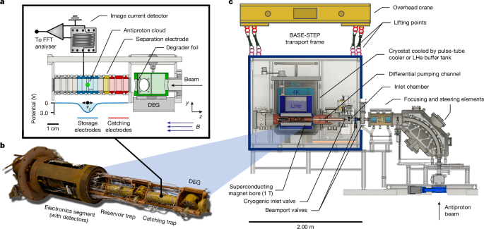
The BASE-STEP catching trap consists of 15 cylindrical electrodes arranged in a coaxial stack (Extended Data Fig. 1a). Sapphire rings provide electrical insulation and mechanical alignment. Antiprotons emerging from the degrader foil follow the magnetic field lines, which have a field strength of B = 993 mT, into the trap.
Three high-voltage electrodes, C01–C03, located on the degrader side capture the antiprotons. Together, these electrodes form a nested axial potential well floated to −142 V with a depth of 16 V (Extended Data Fig. 1b). During capture, a high-voltage switch changes the beam-side electrode C01 from 0 V to −158 V in 30 ns. This pulse closes the potential well centred on C02 and traps antiprotons from the low-energy tail of the degraded beam.
Secondary particles released from the degrader produce cotrapped electrons, which sympathetically cool the antiprotons61. The C02 voltage is then ramped to increase the trapping potential to 200 V. This destabilizes most contaminant negative ions while preserving antiproton confinement because antiprotons have a higher charge-to-mass ratio, q/m.
The trapped particles are subsequently transported to the central region of the catching trap. Electrodes C01–C03 are configured to form a 20 V potential well, and the axial potential is shifted adiabatically through the electrode stack. The typical electrode ramp time is 1 s. The particles are finally confined in a compensated, orthogonal five-electrode Penning trap formed by the central ring electrode C08, correction electrodes C07 and C09, and grounded endcaps beginning at C06 and C10.
Removing Cotrapped Electrons
For nondestructive antiproton detection, residual contaminants must be removed. Otherwise, space-charge effects can distort particle motion and prevent the formation of a stable axial dip signal. The dominant residual species are electrons and H− ions. Because these particles have similar or higher charge-to-mass ratios, high-voltage cleaning cannot remove them selectively.
Cotrapped electrons are removed by applying an axial dipolar drive at 9.59 MHz to an endcap electrode (Extended Data Fig. 2a). The trap depth is first reduced to 1 V, bringing the electron axial frequency into resonance with the applied drive. The trap depth is then reduced further to 0.5 V, evaporating the excited electrons. This sequence is repeated until no electrons remain.
The drive is sufficiently detuned from the motional frequencies of antiprotons and H− ions to avoid unintended excitation. Electron cleaning is repeated after injection when necessary to remove beta-decay-induced electron contamination from activated surfaces (Extended Data Fig. 2b).
The particle cloud is then tuned into resonance with the axial detector at 453 kHz, followed by magnetron sideband cooling. At thermal equilibrium, the interaction between the particles and the detector produces a characteristic dip in the detector noise spectrum.
Removing Heavier Ions and H− Contaminants
Heavier residual ions that remain after the initial high-voltage ramp are removed using stored waveform inverse Fourier transform excitation62 applied to the endcap electrode. The drive spans 20–380 kHz and excites the axial motion of these ions. The trap depth is subsequently reduced to 0.5 V, and the sequence is repeated. This produces a reservoir containing only antiprotons and H− ions.
Antiprotons and H− ions have nearly identical axial frequencies, separated by approximately 250 Hz, and indistinguishable dip widths per particle. Consequently, both species contribute to a combined dip signal. Under the applied catching conditions, the mixed cloud typically contains approximately 80% antiprotons and 20% H− ions.
The two species can be distinguished by their modified cyclotron frequencies, which differ by approximately 16 kHz at B = 993 mT. A single trapped proton is used as a magnetic-field probe before injection, giving:
ν+,p̄ = 15.140 MHz,
ν+,H− = 15.124 MHz.
H− ions are selectively removed by applying a radial dipolar radio-frequency drive to a segmented correction electrode (Extended Data Fig. 2a). A frequency sweep from 15.130 to 15.120 MHz resonantly excites the modified cyclotron motion of H− ions. Their radial amplitudes increase until radial confinement is lost, while the antiprotons remain unaffected.
Successful removal is verified by monitoring the dip width before and after excitation (Extended Data Fig. 2b). The sweep is repeated until the dip width no longer decreases. Although one sweep is typically sufficient, at least three sweeps are applied for robustness. The resulting reservoir contains only antiprotons.
Using this procedure, antiproton reservoirs containing approximately 90 antiprotons are prepared per beam injection.
Particle-Number Calibration
The particle number N, as used in equation (1), is determined from the linear dependence of the axial resonator dip width, Δνz, on the number of trapped particles:
Δνz = Δνz,1N,
where Δνz,1 is the dip width produced by a single particle. Once Δνz,1 has been calibrated, the particle number can be extracted from measured spectra.
Calibration measurements use proton and antiproton clouds of different sizes. Clouds containing approximately 20 particles are prepared in the catching trap. Larger clouds require longer averaging times for precise counting. The clouds are then reduced stepwise to a single particle through controlled evaporation. At each step, spectra are recorded and the dip line shape21 is fitted to determine Δνz.
The final single-particle signal provides the reference value for Δνz,1, allowing particle numbers to be assigned to intermediate cloud sizes. Linear fits of Δνz(N) provide the calibration functions. Proton and antiproton data are treated equivalently because their single-particle dip widths are identical.
Magnetic-Field Dependence of the Dip Width
The dip width depends on the magnetic field because the effective parallel resistance, Rp, of the superconducting resonator varies with field strength. During a magnetic-field ramp from 136 to 993 mT, the dip width decreases (Extended Data Fig. 3a), consistent with a reduction in Rp at higher magnetic fields63.
The single-particle dip width scales linearly with Rp:
Δνz,1 = (1/2π)(q2/(mDz2))Rp.
Separate calibration measurements are therefore performed for each magnetic field. Linear fits at 136 and 993 mT (Extended Data Fig. 3b) give:
Δνz(993 mT) = 3.004(24) Hz · N + 0.129(166) Hz,
Δνz(136 mT) = 3.633(16) Hz · N − 0.017(105) Hz.
The intercepts are consistent with zero within uncertainty. The calibration data were obtained from a proton cloud with N = 21 and an antiproton cloud with N = 18.
The low-particle-number region is especially important because uncertainty in the single-particle reference directly affects the assigned particle numbers. The inset in Extended Data Fig. 3b highlights this region and demonstrates agreement between the particle-number assignment and the linear calibration model.
No direct calibration measurement is available at 880 mT. At this field, the dip width per particle is inferred from the measured detector resistance Rp. Using the proportionality Δνz,1 ∝ Rp and comparisons with calibrated field settings gives:
Δνz,1(880 mT) ≈ 3.07(4) Hz.
Monitoring Particle Number During Storage
The antiproton number in the transport reservoir is monitored over time using an automated measurement sequence that records image-current spectra with an averaging time of 64 s.
The stored antiproton cloud undergoes slow radial expansion, an effect observed and studied in other traps54,64. In general, cylinder-symmetry-breaking electric-field components apply a torque to the trapped ion cloud and drive radial expansion. Possible sources include a small tilt between the electric and magnetic field axes, patch potentials and leakage currents on segmented electrodes.
Radial expansion shifts the axial frequency and increases the dip width because of residual potential imperfections in the trap (Extended Data Fig. 4). In proton tests, radial expansion was not observable over 4 h (ref. 10). The antiproton measurements show faster radial expansion, indicating a larger torque acting on the stored cloud. The origin of this increased torque has not been identified, and the trap configuration has remained unchanged since the proton measurements.
The observed behaviour is consistent with torque-driven radial expansion because the frequency shift can be reset by applying a magnetron cooling drive64. Regular magnetron cooling cycles are therefore required to reset the radial expansion and accurately extract the particle number.
Magnetron sideband cooling is applied at 6-min intervals to suppress this systematic effect and keep the cloud centred in the trap. The remaining drift corresponds to a particle-number offset of only 0.1(2) antiprotons for a cloud containing N = 92.
Additional systematic increases in dip width occur when the tuning ratio and the frequency detuning between the particles and resonator deviate from their optimum values. These parameters are optimized so that their contribution to the particle number is not significant. For substantially larger clouds containing more than 1,000 antiprotons, however, these effects are expected to produce significant uncertainties. In this regime, a rotating-wall drive would be desirable for reliable particle-number determination.
Thirty-Three-Day Particle-Number Record
Over 33 days, more than 26,000 spectra were acquired. The dip width was extracted from each spectrum by fitting the appropriate line shape21. For evaluation, the dip widths were averaged over 24-h intervals, converted using the magnetic-field-dependent calibration functions and rounded to the nearest integer to determine the particle number.
This procedure keeps the statistical deviation from an integer particle number small. Systematic shifts of approximately 0.1 particle numbers therefore do not affect the extracted result.
During the first four days, non-optimized trap parameters caused dip-width broadening and a systematic overestimation of the particle number. These data required an additional correction. After determining the particle number with optimized settings, measurements at 136 and 993 mT were repeated under identical non-optimized conditions and compared with spectra acquired using optimized settings.
The correction factor was defined as:
k = Δνz,true/Δνz,measured.
The resulting values were:
k(993 mT) = 0.9779(11),
k(136 mT) = 0.99395(54).
The evaluation procedure produces the time evolution of the antiproton number shown in Fig. 3 of the main text.
Storage Time and Trap Vacuum Pressure
Only one antiproton was lost during the full 33-day storage period. The loss occurred during voltage-ramp sequences applied to the reservoir as part of manipulation studies. Because the reservoir was monitored only intermittently during these sequences, the precise loss time could not be determined. Based on the available spectrum data, an uncertainty of 3 h was assigned to the loss time.
Using the event timeline in Extended Data Table 1, the total antiproton storage duration was 32 days, 22 h and 38 min. This included:
- 26 days, 13 h and 01 min ± 3 h for N = 92;
- 6 days, 9 h and 37 min ± 3 h for N = 91.
Weighting the storage time by particle number and summing the contributions for N = 92 and N = 91 gives an integrated equivalent single-particle storage time of:
Tp̄ = 8.28025(34) a.
Antiproton Storage-Lifetime Limit
Antiproton annihilation is modelled as a Poisson process:
f(n; λ) = λne−λ/n!,
with expectation value:
λ = Tp̄/τp̄,lower.
Assuming zero observed annihilation events, n = 0, the lower bound on the antiproton lifetime at a specified confidence level is obtained from the probability of observing zero events:
CL = 1 − ε = 1 − f(0; λ),
where:
f(0; λ) = exp(−Tp̄/τp̄,lower).
Under the experimental conditions, this gives a lower limit on the antiproton storage lifetime of:
τp̄,lower = 7.27 a at a 68% confidence level.
Residual-Gas Pressure Limits
The pressure limits reported in the main text are derived by converting the storage lifetime into an upper limit for the partial pressure of a residual gas component. The reaction rate is calculated from the annihilation cross-section:
R = 1/τ = vrel/λ = σngasvrel,
where λ is the mean free path, vrel is the relative velocity between the antiproton and gas molecules, σ is the reaction cross-section and ngas is the gas density.
Using the ideal gas law, the pressure is:
pgas = ngaskBTgas = kBTgas/(τσvrel).
The residual-gas temperature inside the trap chamber is measured using a thermometer on the magnet coil body. Because the coil body has a strong thermal connection to the trap-chamber walls, the gas temperature is typically:
Tgas = 4.3 K.
The analysis assumes that the residual gas consists only of hydrogen molecules and helium atoms. Other gases are assumed to freeze out in the differential-pumping section or trap chamber before reaching the trap centre. Because the residual-gas composition is not known, the upper limit on total pressure is set by the highest partial-pressure limit, assuming that the corresponding component represents 100% of the residual-gas pressure.
Annihilation Cross-Sections
Frequently used cross-section formulas for antiproton annihilation with hydrogen30,40,46,47 originate from studies of protonium formation51,65,66,67 and approximate the reaction as occurring with atomic hydrogen. The cross-section from ref. 66 is:
σ = 3πa02√(E0/E) = 6πa02√(E0/mp̄)(1/vrel),
where a0 is the Bohr radius and E0 = 27.2 eV, twice the binding energy of the hydrogen atom.
Because the cross-section scales as 1/vrel, the reaction rate and the resulting pressure limits are independent of relative velocity. They are therefore also independent of the effective noise temperature of the detection circuit, which defines the velocity of the trapped particle.
The same conclusion applies to helium when the Langevin cross-section is used51. A determination of vrel is therefore unnecessary for reporting the pressure limits in the main text.
Conservative Loss Scenario
A conservative scenario was also considered in which the antiproton loss is attributed to annihilation with residual gas rather than to the voltage ramps used during separation and merging. Under this assumption, a likelihood analysis gives a lower storage-lifetime bound of:
τp̄,lower = 3.6 a at a 68% confidence level.
The maximum-likelihood estimate is 8.3 a. The corresponding pressure constraint relaxes to an upper limit of 4.4 × 10⁻¹⁸ mbar, with a maximum-likelihood value of 1.9 × 10⁻¹⁸ mbar.
This remains below the upper limit quoted in the main text under the assumption of no annihilation events. Even the conservative bound of 4.4 × 10⁻¹⁸ mbar represents, to the authors’ knowledge, the lowest pressure reported for an open cryogenic Penning-trap system and exceeds the minimum operational requirements by more than an order of magnitude.
However, the temporal coincidence between the loss event and the voltage-ramp sequence, together with comparable losses observed for other antiproton clouds under similar manipulation conditions in the same apparatus, makes a chance annihilation event caused by residual gas highly unlikely.
Inlet Valve and Vacuum Interface
The injection beamline operates at local pressures between 6 × 10⁻⁹ and 3 × 10⁻⁸ mbar. These pressures are determined by outgassing, conductance and pumping speed along the beamline.
During trap operation and particle transport, the inlet-chamber pressure is maintained below 1 × 10⁻⁹ mbar using a non-evaporative getter pump. A turbomolecular pump is also used while the valves to the injection beamline are open.
The differential-pumping section, described in ref. 5, connects the inlet-chamber and trap-chamber vacuum systems for antiproton transfer. It has a conductance of 0.16 l s−1 and also manages thermal conductance between the room-temperature and 4 K regions using concentric tubes.
The inlet valve at the entrance of the differential-pumping channel is connected by a copper tube to the 50 K heat shield of the magnet. It is intended to remain open only during antiproton transfer and closed during storage and transport. Closing the valve reduces residual-gas flow into the trap chamber and increases the monolayer formation time.
The inlet valve used in refs. 5 and 10 was replaced with a newly developed version shown in Extended Data Fig. 5. The new design improves sealing, mechanical performance and heat load. In particular, the valve head presses against a polytetrafluoroethylene gasket when closed and is expected to have a lower leak rate than the previously installed metal-on-metal seal.
Autonomous Antiproton Transport Setup
Extended Data Fig. 6 summarizes the electronic system integrated into the transport frame (Fig. 2a) for autonomous operation. The antiproton cloud is confined within the central ring electrode C08 of the catching trap.
Axial confinement is provided by biasing the ring and adjacent correction electrodes with a high-precision voltage supply. All remaining electrodes are grounded through relays at the room-temperature interface.
The antiproton cloud is monitored through the noise spectrum of the image-current detector using a sound-card-based fast Fourier transform system. The cryogenic amplifier is powered by a precision direct-current supply, while the room-temperature amplifiers operate from batteries.
Magnetron sideband cooling is implemented with a waveform generator connected to the radial-excitation line of the catching trap. The transport frame also includes a liquid-helium heater on the liquid-helium tank. The heater increases gas flow for cooling the magnet heat shields by transferring heat to cold gas in heat-exchanger elements on the exhaust line.
Before transport, the turbomolecular-pump gate valve on the inlet chamber is closed, while the non-evaporative getter pump valve remains open to maintain inlet-chamber vacuum conditions. Continuous power is supplied to the getter-pump valve to prevent automatic closure during transport.
All transport electronics, except the room-temperature amplifiers, are powered by a dedicated uninterruptible power supply. The room-temperature amplifiers use separate batteries (Extended Data Fig. 6). The UPS-supported electronics consume approximately 170 W (Extended Data Table 2).
The UPS has a capacity of approximately 750 Wh and provides around 4.5 h of operation after the BASE-STEP apparatus is disconnected from external power.
All voltage supplies, waveform generators, the sound card, sensor-readout devices and telemetry logger are connected to a mini-PC mounted in the transport frame. The transport control computer continuously monitors the particle signal, cryostat temperatures, telemetry sensors, liquid-helium level and vacuum pressures. It also controls electrode voltages and radio-frequency drives for magnetron sideband cooling during transport.
After disconnection from external infrastructure, remote access to the transport control computer is established through a wireless network.
Transport Temperature, Vacuum and Power Measurements
With the cryocooler switched off, the magnet temperature gradually increases (Extended Data Fig. 7a). Once the cryocooler is inactive, the pulse tubes provide a thermal-conduction path to the magnet, which remains thermally linked to the cryocooler. The magnet temperature therefore increases from 4.3 K to an equilibrium value of approximately 5.2 K.
During the 2 h 43 min transport sequence, approximately 11 l of liquid helium evaporated, corresponding to nearly half of the initial liquid-helium buffer reservoir.
The overall temperature evolution during antiproton transport was consistent with that observed during the proton transport rehearsal10. During road transport, between 1.11 and 1.52 h, accelerations of the transport frame, including vibration-induced peaks, generated turbulence in the liquid-helium buffer tank (Extended Data Fig. 7b). This enhanced magnet cooling and maintained the temperature near 4.6 K throughout truck transport.
The transport used a medium-duty truck equipped with air suspension and an automatic transmission. A 5 t steel plate was installed in the truck bed to soften the effective suspension response and reduce mechanical shocks and high-frequency vibrations.
Transient Temperature Spikes
Transient temperature spikes occurred at 2.57 and 2.72 h of autonomous operation. The first spike occurred while the cryocooler flexlines were being connected. During disconnection, a pressure differential developed between the flexlines and the cooling system mounted on the transport frame, with lower pressure in the flexlines. When the lines were reconnected, helium pressure equilibrated and temporarily heated the 4 K stage, producing a short-term increase in magnet temperature.
The second spike occurred when the cryocooler was restarted at the end of transport. While the cryocooler was inactive, helium gas inside it warmed. Initial compressor operation consequently transferred heat into the 4 K stage before steady-state cooling resumed. After the cooler restarted, the magnet temperature returned to its initial operating value.
UPS Capacity and Vacuum Stability
Approximately 50% of the UPS battery capacity was consumed during transport. During stationary periods, the UPS was temporarily reconnected to external power to preserve battery capacity.
Vacuum conditions remained stable throughout transport. Pressure spikes reaching the 10−7-mbar level were observed in the cryostat vacuum chamber and were attributed to gas release from the multilayer insulation surrounding the magnet’s thermal stages.
By contrast, the inlet-chamber pressure remained below the gauge detection threshold of 1 × 10⁻⁹ mbar. Only occasional vibration-induced outgassing spikes were observed, and these remained below 3 × 10⁻⁹ mbar.
Source: www.nature.com