


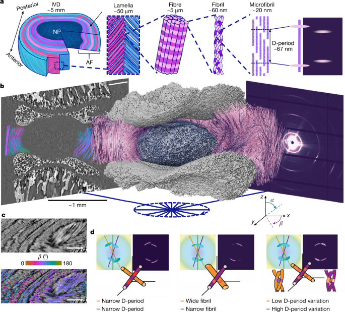
The study describes a multimodal imaging and analysis workflow for measuring collagen-fibre structure and nanoscale deformation inside intervertebral discs (IVDs). The researchers combined synchrotron tomographic small-angle X-ray scattering (SAXS), phase-contrast computed tomography (pCT), in situ mechanical loading, fibre tracing and digital volume correlation (DVC). They developed the TomoSAXS software pipeline to associate collagen diffraction signals with individual fibres and estimate properties such as collagen D-period, D-period variation, fibril radius and nanoscale strain before and after compression.
Sample preparation
Samples came from male Sprague Dawley rats aged eight weeks. The animals were housed at the University of Manchester Biomedical Sciences Facility under controlled conditions, with 12-hour light–dark cycles, a temperature of 22 °C and unrestricted access to food and water. Tissue collection complied with the UK Animals (Scientific Procedures) Act 1986 and local UK Home Office regulations. Institutional approval was granted by the University of Manchester Animal Welfare and Ethics Review Board under Home Office Licence #70/8858 or I045CA465. No randomization or blinding was performed.
Whole spines were dissected, snap-frozen in liquid nitrogen and stored at −80 °C. Thawing and further dissection were completed within 24 hours of each experiment, following the procedure described by Parmenter et al.22. The resulting samples were whole IVDs from thoracic vertebra 10 through lumbar vertebra 2, with half of the adjacent vertebrae retained on either side.
Each sample was attached to a resin-printed holder with cyanoacrylate glue (VetBond; 3M Science). The specimens were aligned so that the central transverse plane of the IVD was parallel to the loading plates. A Kapton polyimide tube surrounded each specimen, leaving approximately 0.5 mm exposed.
The holders were mounted in a Deben CT500 micromechanical tester equipped with a 100 N load cell, specified to have ±1% accuracy. The tester used a custom open-frame design described previously22. Displacement was measured with a 10 mm extensometer with 3 µm resolution and 1% linearity. The open frame supported sample alignment and hydration while reducing obstruction of the X-ray beam during SAXS measurements.
Samples were kept hydrated by immersion in phosphate-buffered saline (PBS). PBS was delivered through a capillary at the base of the holder from a 100 ml syringe connected to a stopped-flow module (Bio-Logic). Continuous flow maintained the fluid level despite minor leakage from the 3D-printed holder.
Sequential SAXS and pCT experiment
Simultaneous SAXS and pCT would have been preferable, but Diamond Light Source (DLS) did not have a dedicated SAXS–pCT beamline for the experiment. The researchers therefore used a sequential protocol: preloaded SAXS at beamline I22, preloaded pCT at beamline I13, loaded pCT at I13, and loaded SAXS at I22. Stabilized sample holders and identical mechanical rigs at both beamlines were used to improve comparability.
Tomographic SAXS acquisition
SAXS data were collected at the I22 beamline at DLS during experiment SM29784-8, from 12 to 15 December 2023. A Deben CT500 was mounted on a rotation stage above the sample table. A Dectris Pilatus P3-2M detector was positioned 9 m from the stage, with a vacuum tube between the sample and detector to reduce air scattering.
All SAXS measurements used a 14 keV beam with a 20 µm beam size. Each sample was first mapped at 0° using a raster scan of approximately 100 × 100 SAXS frames. The exposure time was 50 ms and the step size was 20 µm. These maps were inspected to locate the IVD, after which a 5 × 1 mm region of interest was selected for tomographic SAXS.
Tomographic scans covered raster maps of approximately 250 × 10 SAXS frames, with a 20 µm step size and 150 ms exposure time. Measurements were made at nine equally spaced angular orientations, separated by 22.5°, between −85° and 95°. This range reduced blocking by the mechanical support rods. A complete single-axis SAXS tomography delivered a radiation dose of 12.2 kGy.
The relatively large 22.5° angular step was necessary because the ring current had fallen to 200 mA during the beamtime, substantially reducing the available flux. The method could be adapted to smaller angular steps, which would increase the fraction of fibres intersecting the Ewald sphere. SAXS data for one horizontal slice are available in the Supplementary Dataset59.
pCT acquisition and reconstruction
pCT was performed at the Diamond–Manchester Imaging Branchline I13-2 at DLS during experiment SM29784-9, from 12 to 14 December 2023. The setup followed established protocols22, using a mean energy of 27.6 keV, 1,800 projections and a 0.5 m sample-to-detector distance. The exposure time was 0.15 s to account for the reduced ring current.
The insertion-device gap was set to 5 mm during scanning and increased to 7 mm for alignment and low-resolution scans to reduce radiation dose. Initial scans used a 1.25× objective, producing 2.6 µm voxels and a 6.7 × 5.6 mm field of view. These scans captured the sample environment, including the Kapton tube needed for SAXS co-registration.
Additional scans before and after compression used a 2× objective, producing 1.625 µm voxels with a 4.2 × 3.5 mm field of view. Radiation doses were 1.35 kGy per scan at 2.6 µm voxel size and 27 kGy per scan at 1.625 µm voxel size. Tomograms were reconstructed with the open-source Python library Savu 4.2 and further processed in ImageJ 1.54 as described previously22. Images of IVD1 are available in Supplementary Dataset60.
In situ mechanical testing
Samples were scanned while under axial compression applied along the laboratory vertical z-direction. Two identical Deben CT500 rigs with 100 N load cells were used: one at I22, supplied by Imperial College London, and one at I13-2, supplied by the University of Manchester at Harwell.
At I22, a 1 N preload was applied before SAXS scanning. This corresponded to approximately 40% of the animals’ body weight, which was 260 ± 33 g, and prevented excessive swelling of the nucleus pulposus. Samples were allowed to relax for 20 minutes before scanning. This interval was selected because the load readings had stabilized, changing by less than 0.01 N in one minute.
After SAXS, samples were clamped in place with bespoke 3D-printed holders and screws and transferred to I13-2. The clamped samples were secured at the top of the second mechanical rig. Its bottom platen was slowly raised until the screw holes in the rig aligned with those in the sample holder, which was then fixed in place. The clamps were removed before the preload pCT scans.
After the first pCT scan at a 1.6 µm voxel size, the bottom platen was displaced by 50 µm along the laboratory z-direction. This reduced IVD height by 2–5%, depending on the sample. Axial compression was selected because it simplified both the experiment and the interpretation. Samples were again allowed at least 20 minutes for stress relaxation before scanning.
Following imaging, each sample was clamped in its loaded state, removed from the rig and returned to I22. The sample was placed back into the mechanical tester, the clamps were removed and loaded SAXS scans were collected using the same protocol as the initial scans.
Fibre tracing and DVC analysis
Fibres were traced in the 1.6 µm preload images with the Avizo XFiber module in Avizo 3D 2023.2. Parameters are provided in Supplementary Note 3. Fibres clearly associated with imaging artefacts, including mineralized-tissue streaks and reconstruction ring artefacts, were removed. Fibre spatial graphs were exported as XML files, and each fibre identification number was retained throughout the subsequent analysis.
Fibre orientation and curvature were calculated from a three-dimensional polynomial fit to each traced fibre centreline using a custom MATLAB R2023a script available at github.com/DiamondLightSource/tomosaxs. The analysis produced fibre ID, x, y, z, curvature, α-orientation and β-orientation values at points spaced every 6.5 µm along each fibre. Fibre IDs and orientation values were converted into three-dimensional volume images for TomoSAXS reconstruction.
Curvature, k(s), was calculated from the first and second derivatives of the fitted curve:
k(s) = ||r′(s) × r″(s)|| / ||r′(s)||3.
Local DVC analysis was performed with the open-source iDVC software, available at tomographicimaging.github.io/iDVC/4,21–24,61. The fibre coordinates were used as a point cloud defining the locations of the tracked sub-volumes. Each sample contained 0.7–1.4 million DVC measurement points, according to Supplementary Table 1.
Spherical sub-volumes 40 voxels in diameter, equivalent to 65 µm, were matched between preload and loaded images using a zero-normalized sum-of-squares difference function. The matching allowed 12 degrees of freedom, including translation, rotation and first-order strain. Six thousand sampling points were used within each sub-volume. The displacement of the first point in the cloud was established by manually tracking a landmark between the preload and loaded images in ImageJ.
Two strain methods were applied to the DVC displacement fields to probe different length scales. Tissue-level strains were calculated by differentiating a polynomial fit to the displacement field and deriving the Lagrangian strain tensor at each point61. The 75 closest points to each measurement point were used for fitting to reduce noise and improve accuracy.
The first principal strain was obtained from the maximum positive eigenvalue, while the third principal strain was obtained from the maximum negative eigenvalue. The angle between each corresponding eigenvector and the local fibre direction was expressed from 0°—parallel to the fibre—to 90°—orthogonal to the fibre. Radial and circumferential strains were calculated by projecting the strain tensor onto the local radial and circumferential directions. Fibre strains were calculated with a custom MATLAB R2023a script by fitting a polynomial to displacement along each fibre.
The double-projection zero-strain method22 was used to assess DVC accuracy. The mean absolute error for zero-strain displacement was 88.5 nm, with a precision of 83.5 nm based on the standard deviation of the absolute error. Tissue-level accuracy and precision were both 0.16%. Fibre-level accuracy was 0.08% and precision was 0.10%.
For a simulated 10% compression, DVC displacement accuracy was 198 nm, tissue-strain accuracy was 0.40% and fibre-strain accuracy was 0.45%.
To calculate the orientation of the same fibres after loading, DVC displacements were applied to the fibre points in MATLAB. The orientations of the deformed fibres were then calculated, and loaded fibre-ID, α and β volume images were generated for TomoSAXS reconstruction.
Three-dimensional diffraction modelling
The researchers modelled three-dimensional diffraction by simulating the meridional X-ray diffraction peaks of collagen fibrils with nanoscale fibre symmetry. The model accepted user-defined wavelength, lattice spacing and angular tilt values and accounted for the changing intersection between the three-dimensional scattering intensity and the Ewald sphere.
The implementation was written in a custom Python library available at github.com/DiamondLightSource/tomosaxs. It extends the model described by Badar et al.1. Meridional scattering caused by collagen D-periodicity was represented by a series of three-dimensional, semi-flat ellipsoidal functions. Their positions were set at harmonics of the inverse D-period, q0n = 2πn/D.
The radial width in reciprocal space, wa, represented heterogeneity in fibril pre-strain. The angular width, wμ, represented the inverse fibril diameter and intrafibrillar tilting. The ellipsoid’s degree of circularity, δ, ranged from 0 for a straight function to 1 for a circular ellipsoid.
A semi-flat rather than completely flat meridional ellipsoid was used because the meridional ellipse showed some arcing even in tissue with uniaxial fibril orientation. The researchers suggested that this may be related to intrafibrillar tilting of the microfibrils38.
Because the Ewald sphere has a radius proportional to 1/λ, both the intensity and pattern of the two-dimensional fibril diffraction depend on the fibre’s three-dimensional α and β tilt angles and on the beam wavelength. The model could calculate fibril scattering in two dimensions or produce one-dimensional azimuthal (χ) and radial (q) profiles by averaging along the complementary axis.
The TomoSAXS workflow
The diffraction model was combined with pCT or DVC data containing the α and β fibre orientations to reconstruct the third-order collagen diffraction peak. This peak typically had intensity between wavevectors of approximately 0.26 and 0.32 nm−1. TomoSAXS was implemented as five discrete modules in Python 3.10.
Module 1: spatial co-registration
The first module spatially registered the pCT and SAXS scans and identified the collagen fibres intersecting each SAXS beam path at every tomographic rotation.
Module 2: background correction
The second module corrected SAXS signals for scattering from PBS, the Kapton tube and air. It built on the adcorr Python package62. Because the pCT and SAXS datasets were co-registered, the method used the changing sample thickness along each beam path to adjust the relative contributions of dispersant and sample rather than assuming a uniform thickness.
Module 3: SAXS amplitude estimation
The third module used singular-value decomposition (SVD) and the three-dimensional diffraction model to make initial estimates of the SAXS amplitude for individual fibres. These estimates identified strongly scattering fibres that could be solved individually in the next stage.
Module 4: iterative fibre fitting
The fourth module was the core reconstruction stage. It scanned SAXS tomography data across azimuthal χ and rotation axes to identify sectors in which one, two or three fibres dominated the scattering. A fibre was considered isolated when it contributed more than 90% of the total scattering across at least a 10° sector around the circumferential χ axis.
Within each sector, radial intensity profiles were calculated at three equally spaced angular positions. Three-dimensional diffraction models were then fitted to estimate the mean collagen D-period, variation in D-period and fibril radius. For double- and triple-fibre fits, the algorithm required at least 5° of angular separation between fibres and minimum predicted intensity from each fibre to prevent degenerate fits.
The fitting used two stages. First, the algorithm searched all rotations and beam paths for sufficiently independent single-fibre signals until no additional single fibres could be solved. It then repeated the process using single, double and triple fibre fits, iterating through all angles and rotations until no additional fibres could be resolved.
Module 5: spatial reconstruction
The fifth module spatially reconstructed the fitted nanoscale metrics and estimated fibril-level strain during loading. DVC measurements of microscale deformation were used to locate the same fibre in the unloaded and loaded datasets.
Registration and background correction
Co-registration used fiducial features visible in both modalities. The Kapton tube provided horizontal alignment, while the mineralized vertebral endplates provided vertical alignment. The 1.625 µm pCT images did not contain enough of the Kapton tube for direct registration, so they were registered to the 2.6 µm images.
Both pCT datasets were downsampled to 6.5 µm voxels, and the offset between them was calculated in the x, y and z directions. Fibre-orientation TIFF stacks, with an absolute voxel size of 8.125 µm, were padded to the original high-resolution reconstruction size of 512 × 512 × 432 voxels and centred using the offset between the high- and low-resolution images.
Vertical registration between SAXS and pCT used the mineralized endplate boundaries in the 0° SAXS intensity map and the corresponding two-dimensional total phase-contrast intensity maps from pCT. Horizontal registration used characteristic SAXS peaks from the Kapton tube and manual segmentation of the tube in pCT.
For each of the nine SAXS orientations, spanning −90° to 90°, fibre orientation, fibre-index and Kapton data from vertically isolated SAXS slices were rotated to the corresponding angle. The left edge of the Kapton tube was then aligned between SAXS and pCT. This identified the indexed fibres contributing to the SAXS signal along each raster-scan beam path.
For every frame, the analysis recorded each fibre’s orientation, index and number of CT voxels along its beam path. It also calculated the distance between each fibre and the centre of the beam path, which was used as a weighting factor during model fitting. The total specimen thickness along each beam path was also calculated.
Background correction followed the approach of Pauw et al.62. Separate scans using the SAXS tomography settings were collected for an empty Kapton tube and for a Kapton tube filled with PBS. These measurements represented scattering from the holder and dispersant. The signals were subtracted from each sample frame with the adcorr library, while the sample-to-dispersant ratio was adjusted according to the frame-specific sample thickness. Corrected data were saved as HDF5 files for each TomoSAXS slice.
Estimating fibre amplitudes and fitting diffraction peaks
For the initial amplitude estimate, the analysis used a common mean value for other peak properties, including peak position and radial and angular widths. This was justified by the limited variation in peak position observed in two-dimensional data.
At sample position x and rotation angle r, the angular intensity of the third-order collagen peak was represented as the sum of the contributions from all fibres in the volume:
Ixr(χ) = Σi wiIir(χ; q0, Δq0, α, β).
The weighting factor was zero for fibres outside the beam path and otherwise proportional to the intensity at the fibre location, assuming a known Gaussian beam profile. Since the initial step used common average peak parameters, each fibre contribution could be calculated up to an amplitude factor. The resulting overdetermined linear system was solved with SVD.
A Python dictionary was created for each SAXS frame. It contained 0–180° angular intensity values, obtained by radial integration between 0.26 and 0.32 nm−1 and binned into 36 averaged χ points. The data were smoothed with a one-dimensional Savitzky–Golay filter using a window length of 9 and polynomial order 1.
One matrix contained the concatenated measured angular integrations, while a second contained the predicted contribution of every fibre to the same intervals. Fibre amplitudes were estimated through non-negative linear least-squares regression. Each fibre entry stored its index, α and β angles and a space for fitted nanoscale parameters.
Single- and multiple-fibre fitting
Initial simulated angular profiles used the estimated amplitudes and the orientation-specific fibre dictionaries. Fibre contributions were weighted according to their distance from the beam centre, using:
weighting factor = exp(−d2 / 2w2),
where d is the distance from the beam centre and w is the beam diameter. The model used pCT-derived tilt angles and average nanoscale parameters of q0 = 0.2856 nm−1, wa = 0.005 nm−1, wμ = 0.2 nm−1 and δ = 0.5. The rationale for these values is provided in Supplementary Note 14.
Single-fibre fits
For each fibre in each beam path and rotation, the algorithm calculated its individual angular contribution to the total signal. A fibre was identified as dominant when its contribution exceeded 90% of the total intensity throughout a 10° angular interval. The fibre index, beam-path location and angular sector were recorded.
For each candidate, three equally spaced radial slices were calculated across the sector, using a default slice width of 6°. These profiles were fitted simultaneously with three-dimensional diffraction models using the minimize() function in the lmfit Python library and the Nelder–Mead algorithm.
The α and β angles and the fibre weighting factor were fixed. The fitted parameters were q0, wa, wμ, amplitude and δ. Fits had to meet thresholds for parameter values and statistical quality, including a standard-error threshold of 25%. Successful fits were added to the corresponding fibre entry, while unsuccessful fits were stored separately and excluded from later analysis.
Once a fibre had been fitted, its contribution could be removed from other beam paths where it occurred. The algorithm therefore repeated the search until no further independently scattering single fibres could be identified. This first stage isolated the strongest signals, representing approximately 10–20% of indexed fibres per slice, and provided robust fits for subsequent deconvolution.
Overlapping fibres
The next stage fitted cases in which two or three fibres together produced a sufficiently independent signal. For a pair of fibres, their combined contribution had to exceed 95% of the total signal across a 10° sector.
Validation simulations showed that a dominant fibre could bias the fitted parameters of the other fibre or fibres. Therefore, each fibre in a pair had to contribute at least 20% of the total scattering across more than 90% of the sector. Qualifying pairs were fitted with the same minimization procedure. After every fit, the parameter database was updated and the angular profiles were rescanned for newly solvable single, double or triple fibre instances.
The process was repeated across all beam paths and rotations for a maximum of 10 loops. The procedure stopped earlier if a loop produced no increase in the number of fitted fibres.
The complete TomoSAXS workflow was run separately for each horizontal 20 µm SAXS tomography slice on the DLS computing cluster. Individual slices were processed in parallel. The five-module process took 6–7 days, with each module triggered separately and iteratively. TomoSAXS fitting took 4–5 days and produced fits for a mean of 60.08% of fibres per slice.
This percentage includes multiple fits for individual fibres appearing in different TomoSAXS slices. It does not represent the proportion of the total sample volume fitted, because TomoSAXS operates on individual fibres rather than voxels, unlike SAXS-TT28. Reconstruction quality was spatially heterogeneous and depended on the density and orientation of fibres in each slice.
Reconstructing nanoscale metrics and strain
After fitting, the estimated parameters were mapped back into three-dimensional space. For each parameter, blank maps matching the fibre-index maps were created, and the fitted value was assigned to every voxel belonging to a solved fibre.
When a fibre had fitted values in multiple TomoSAXS slices, missing values between fitted slices were estimated by linear interpolation, provided that the unfitted slices lay between two fitted points.
To estimate nanoscale strain during compression, fibres with fits in both unloaded and loaded datasets were selected. The DVC-derived vertical deformation was used to estimate the corresponding position in the loaded TomoSAXS scan. Strain in each nanoscale parameter was calculated as the percentage difference between its unloaded and loaded fitted values.
Digital-phantom validation
The spatial calibration between pCT and SAXS enabled accuracy testing with digital phantoms. Known artificial nanoscale parameters were assigned to each indexed fibre in each TomoSAXS slice while preserving fibre orientation, initial scattering amplitude and per-instance weighting.
Experimental noise was added to the simulated SAXS data. The accuracy and precision of the recovered nanoscale parameters were then calculated as the mean absolute error and the standard deviation of the absolute error.
Laboratory TomoSAXS demonstration
Chicken foot tendons were dissected and air-cured under tare loads of 0.5 N, 1.5 N and 3.5 N to generate different levels of collagen pre-strain. Three tendons were arranged at different overlapping orientations and attached to a 3D-printed holder with superglue.
SAXS scans were performed with a Xenocs Xeuss 3.0 at DLS using a 400 µm beam and a 5-minute exposure. Nine angular rotations between 0° and 180° were collected, with 11 beam paths at each rotation. Micro-computed tomography was performed with a Phoenix V|tome|x system at the Research Complex at Harwell using 14.3 µm voxels.
The collagen fibrils in each tendon were assumed to align with the tendon’s principal axis. For this proof-of-concept experiment, the sample was divided into an 11 × 11 grid rather than being reconstructed fibre by fibre. The TomoSAXS reconstruction used modules 4 and 5, without the background correction or SVD-based scattering-amplitude estimation used in the full pipeline.
Human IVD imaging
A whole formalin-fixed human IVD from spinal level thoracic 11–12 was imaged. The donor was a 64-year-old man with no known spinal pathologies. Donation and dissection were carried out at the Laboratoire d’Anatomie des Alpes Françaises in November 2023 under French body-donation legislation. Transport and imaging were approved by the UK Health Research Authority through the Integrated Research Application System, approval #200429, and by the French Ministry of Health.
Static imaging was performed at the BM18 beamline of the European Synchrotron Radiation Facility (ESRF) using hierarchical pCT45. The complete IVD was captured at 10 µm voxel size, and a central local-zoom scan at 4 µm was used to visualize collagen fibres throughout the organ.
Fibre tracing was performed on the 10 µm scan with the Avizo XFiber module in Avizo 3D 2023.2. Correlative high-energy tomographic SAXS was performed at ESRF beamline ID31 using a 75 keV beam, a 100 µm beam size and 24 angular positions.
A modified TomoSAXS pipeline was needed for a single human IVD slice because the sample volume was approximately 103 times larger and contained many more fibres per beam path. First, α and β fibre-angle maps were independently quantized by applying k-means clustering to non-zero angles rounded to 3° increments. The maps were then combined pixel by pixel into a three-dimensional orientation-label map. This reduced the number of fibre indices from more than 26,000 to approximately 3,600.
Second, the multiple-fibre fitting procedure was extended to include four- and five-fibre clusters across the χ axis. Third, parallel processing was introduced to handle the larger number of beam paths and indexed objects. Instead of processing rotations sequentially, the rotations were processed in parallel on a computing cluster, with all rotations reading from and updating a shared database of fitted fibres. Further details are provided in Supplementary Note 22.
Statistical analysis
Two-sided ordinary least-squares regression was used to assess agreement between known and estimated properties in digital-phantom data, both with and without experimental noise. Correlations between per-fibre mean values of fibre strain, D-period, D-period variation and D-period strain were also tested with ordinary least-squares regression. No adjustments were made for multiple comparisons.
Source: www.nature.com