


Study design
This study used samples from the Lifelines NEXT (LLNEXT) birth cohort, which investigates intrinsic and environmental factors that influence health and disease across four generations23. LLNEXT is part of the Lifelines (LL) cohort, a prospective, population-based study involving 167,729 people from three generations living in the northern Netherlands56,57.
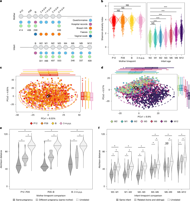
Between 2016 and 2023, 1,452 pregnant women, their partners and infants were enrolled in LLNEXT and followed until at least 1 year after birth. Participants provided multiple biological samples, including faeces, breast milk and vaginal swabs. Medical, lifestyle, social and environmental information was collected through questionnaires completed at 14 timepoints and through connected devices.
The LLNEXT study was approved by the Ethics Committee of the University Medical Center Groningen (UMCG; METc2015/600). All participants, or their parents or legal guardians, provided written informed consent. The present analysis included the first 714 mother–infant pairs recruited between 2016 and 2019.
Predictors
Predictor information was obtained from LLNEXT and, when parents were enrolled, the LL cohort. Questionnaire data and medical records were integrated to improve completeness. Maternal predictors covered the period before conception, pregnancy, delivery and the postpartum period, while infant predictors were collected at birth and throughout the first year of life.
Predictors were analysed either cross-sectionally, including static variables such as delivery mode (n = 316; Supplementary Table 1), or longitudinally, including time-varying variables such as feeding mode (n = 158; Supplementary Table 2).
Pre-pregnancy predictors
Maternal pre-pregnancy body mass index (BMI; kg m−2) was obtained from the LL cohort and supplemented with LLNEXT medical records. Measurements from as far as 8 years before conception were included.
Maternal smoking history was classified as positive when a participant reported smoking continuously for at least 1 year at any time in her life. Among the LLNEXT mothers, smoking occurred between 10 and 29 years of age, with a median starting age of 15 years.
Pregnancy and delivery predictors
Maternal education and monthly income were recorded at 18 weeks of pregnancy (P18). Education was grouped into elementary or lower-secondary, upper-secondary or tertiary education categories58. Monthly income was estimated using data from the Dutch Social and Cultural Planning Office59 and classified as low (<€800–1,800), middle (€1,800–2,400) or high (>€2,400). Questionnaires completed at P18 also covered reproductive and dental health and substance use.
Maternal food preferences and avoidances were assessed at 12 and 32 weeks of pregnancy (P12 and P32) using a 94-item questionnaire developed by Wageningen University & Research (WUR). Each item was scored from 0, indicating strong aversion, to 10, indicating strong preference. Because responses were highly correlated between timepoints (r > 0.8), the datasets were combined. Missing values were imputed using linear regression between the two timepoints.
Delivery information was obtained from medical records, including birth cards completed by midwives or obstetricians in hospital or at home, and participant questionnaires. Variables included delivery mode, delivery location and duration, medication use during pregnancy and pregnancy complications.
Postpartum predictors
At 2 months postpartum (M2), maternal diet was assessed with a self-administered, semi-quantitative Dutch food-frequency questionnaire (FFQ) containing 177 food items (Supplementary Table 72). Trained WUR research dieticians quality-checked the FFQs, which covered dietary intake during the preceding month. Mothers reported consumption from never to 7 days per week.
Portion sizes were estimated in grams per day using natural portions and household measures from the ‘Measures, Weights and Codes’ booklet60. Daily energy intake was calculated from consumption frequency, portion size and energy values in the 2006 Dutch food composition table (NEVO; RIVM)61. Six mothers reporting fewer than 500 kcal or more than 4,000 kcal per day were excluded.
Food items were grouped into 28 broad categories (Supplementary Table 72), named after the most abundant items in each group. An alternative Mediterranean diet quality score was also calculated62. Dietary patterns were identified through unsupervised hierarchical clustering of food groups measured in grams per day. Euclidean distances and complete-linkage clustering were used. After comparing different clustering heights, a dendrogram supported a cut height of 26, producing 10 clusters. Cluster centroids represented the average consumption of each variable within a cluster. Analyses were conducted with the dendextend package (v.1.17.1)63 in R.
Infant predictors
Infant stool consistency was assessed with the Brussels Infants and Toddlers Stool Scale (BITSS)64 at 2 weeks and 1, 2, 3, 6, 9 and 12 months. Stool features and gastrointestinal (GI) symptoms were collected with the validated ROME IV questionnaire65 at 1, 2, 3, 6, 9 and 12 months.
Parent-perceived GI function, distress and feeding tolerance were measured at 3 and 12 months using the 13-item Infant Gastrointestinal Symptom Questionnaire (IGSQ). Items were scored according to the user guidelines and combined into a composite score66. Because scores were right-skewed, infants were classified at each timepoint according to the population median. Scores at or below the median indicated no or little GI distress, while higher scores indicated medium-to-high distress.
Infant feeding mode and dietary intake were obtained from birth cards and infant FFQs. Parents or guardians completed Dutch infant FFQs covering the preceding month at 6 months (49 items), 9 months (66 items) and 12 months (66 items) (Supplementary Table 37). These questionnaires were quality-checked by trained WUR research dieticians.
Feeding mode immediately after birth was classified as breastfeeding, mixed feeding or formula feeding (FF). Mixed feeding was defined as any combination of breast milk and formula. Feeding mode after birth was analysed longitudinally, with missing values imputed where possible from feeding patterns between 2 weeks and 3 months. For example, patterns such as FF–NA–FF–FF and FF–FF–NA–FF were classified as formula feeding at all available timepoints between 2 weeks and 3 months.
Complementary feeding was defined using food items from the 6-, 9- and 12-month FFQs and the CDC definition: “foods or drinks other than breast milk or infant formula (e.g. infant cereals, fruits, vegetables, water)”. Consumption frequency ranged from never to 7 days per week. Portion sizes were estimated in grams per day using the ‘Measures, Weights and Codes’ booklet67, and energy intake was calculated using the 2006 NEVO food composition table61.
Because breast milk intake cannot be measured accurately in grams or calories, total daily intake and energy intake included complementary foods only and excluded breast milk and formula. Macronutrients were converted to energy percentages using 4 kcal g−1 for carbohydrates and protein, 9 kcal g−1 for fat and 2 kcal g−1 for fibre.
Food items were grouped into 19 categories at 6 months and 22 categories at 9 and 12 months (Supplementary Table 37). Dairy and fruit were analysed both separately and as grouped categories. Consumption was recorded as yes or no and as weighted frequency, with 1 day per week equivalent to 0.04 when a month was defined as 28 days.
Infant dietary patterns at 6, 9 and 12 months were derived through factor analysis (FA), using principal-component extraction of standardized FFQ items measured in grams per day. Bartlett’s test of sphericity and the Kaiser–Meyer–Olkin test confirmed that the data were suitable for FA; all Kaiser–Meyer–Olkin values exceeded 0.5. Components with eigenvalues ≥ 1.5 and those supported by the scree-plot elbow were retained and orthogonally rotated using varimax rotation. Food items with loadings |>0.35| were considered important contributors. Component scores were calculated using the regression method68. Statistical tests used the psych package (v.2.2.9)69, and FA was performed with the factanal function in the stats package (v.4.2.1)70 in R.
Infant weight, length and head circumference were collected from medical records, growth charts and questionnaires between birth and 12 months. Missing measurements were estimated using third-degree polynomial regressions for each anthropometric variable. Standard deviation scores were calculated with the Growth Analyzer Research Calculation Tool (v4.1), using the Fifth Dutch Growth Study from 2008–2009 as the reference71.
Infant development was evaluated at 6 and 12 months using the 30-item Ages and Stages Questionnaire, third edition (ASQ-3). Total scores ranged from 0 to 300, while communication, gross motor, fine motor, problem-solving and personal–social domains each ranged from 0 to 60. Scores were calculated according to the ASQ-3 User’s Guide72, including its procedures for handling missing data. Development was classified as typical or delayed using relaxed and strict domain-specific thresholds. ASQ-6 included infants aged 5–7 months and ASQ-12 included infants aged 11–13 months.
Infant health data were obtained from general health questionnaires at 4 and 12 months, food-allergy questionnaires at 4, 6, 9 and 12 months, and the International Study of Asthma and Allergies in Childhood (ISAAC) questionnaire73 at 12 months.
Atopic dermatitis, referred to here as eczema, was assessed by research nurses at 3 and 12 months using the SCORing Atopic Dermatitis (SCORAD) method74. SCORAD evaluates affected skin area, itching, sleeplessness and related symptoms, producing a maximum score of 83. Eczema was defined using three variables: parent-reported eczema, strict diagnosis and relaxed diagnosis. Under the latter two definitions, eczema was recorded when the infant used eczema medication between 2 weeks and 12 months, the parents reported eczema, or the objective SCORAD score was >0.
For the strict definition, controls had no eczema medication use, no parental report of eczema and an objective SCORAD score of 0. The relaxed control group additionally incorporated information from the parent questionnaire definition.
Infant crying was assessed at 2 weeks and 1, 2, 3, 6, 9 and 12 months using an 11-item questionnaire validated for Dutch infants75. Sleep was assessed at 3, 6 and 12 months using the 13-item Brief Infant Sleep Questionnaire (BISQ)76.
Parents reported infant medication use at 2 weeks and 1, 2, 3, 6, 9 and 12 months. These data were supplemented with medication information from other LLNEXT questionnaires. The in-house SORTA tool (System for Ontology-based Re-coding and Technical Annotation)77 semi-automatically linked textual medication reports to Anatomical Therapeutic Chemical codes. Unmatched medications were manually curated. Medication variables were analysed cumulatively, indicating whether the infant had ever received a specified medication up to each timepoint.
Other predictors across pregnancy, delivery and postpartum
Information about family pets was combined from maternal questionnaires at P18, P32, 1 month postpartum and 4 months postpartum, together with infant questionnaires at 4 and 12 months. Family living circumstances were obtained from maternal questionnaires at P32 and 4 months postpartum and classified as house, farm, flat or other.
Maternal stool consistency was measured with the Bristol Stool Scale at P12, P28, delivery and 3 months postpartum. The validated ROME III questionnaire78, completed at P28 and 3 months postpartum, was used to identify functional gastrointestinal disorders (FGIDs). Mothers were classified as having no FGID, irritable bowel syndrome, functional constipation or functional bloating. Stool frequency and maternal GI health diary data were also derived from these assessments.
Maternal medication use was self-reported at P28, delivery and 3 months postpartum. As for infant medication data, SORTA was used to link written medication descriptions to Anatomical Therapeutic Chemical codes, followed by manual curation of unmatched entries.
Maternal stress during the preceding year was measured at 1 and 10 months postpartum with the 12-item Long-term Difficulties Inventory (LDI)79. Work, home, family and other stressful situations were rated as not stressful (0), somewhat stressful (1) or very stressful (2). Item scores were summed and averaged to generate pregnancy and post-pregnancy stress scores.
Correlations between predictors
Spearman correlation coefficients were calculated for all predictors (Supplementary Tables 73–76). To limit collinearity in subsequent analyses, predictors with correlations above 0.7 or below −0.7 and an FDR < 0.05 were excluded. Removed variables included selected maternal and infant diet measures, growth measurements and ASQ variables.
Sample collection
Faecal samples
A total of 1,587 maternal and 2,939 infant faecal samples from 714 mother–infant pairs were collected and successfully sequenced across 10 timepoints.
Maternal samples were collected at P12 (n = 414), P28 (n = 406), delivery (n = 268) and 3 months postpartum (n = 499; Supplementary Tables 12 and 13). Infant samples were collected at 2 weeks (n = 331), 1 month (n = 466), 2 months (n = 497), 3 months (n = 553), 6 months (n = 346), 9 months (n = 337) and 12 months (n = 409), averaging four samples per infant.
Infant sampling windows were day 3–22 for 2 weeks, day 23–45 for 1 month, day 46–77 for 2 months, day 78–143 for 3 months, day 148–232 for 6 months, day 244–329 for 9 months and day 335–436 for 12 months. Meconium samples were excluded because their low microbial biomass did not yield viable microbial reads, consistent with previous findings20.
Parents used UMCG stool collection kits and froze samples at home at −20 °C within 10 min of stool production20. UMCG personnel transported the samples in portable freezers. Samples were stored at −20 °C for short-term storage or −80 °C for long-term storage until DNA extraction.
Human breast milk samples
Mothers expressed breast milk using their usual breast pump without specially cleaning the breast tissue. They were asked to pump from one breast, preferably the right, during the second feed after midnight and at least 2 h after the previous feed from that breast.
Milk was gently mixed, and 2 ml aliquots were transferred to cryotubes using plastic dropper pipettes (H10041, MLS). Samples were frozen at −20 °C at home, transported to the laboratory in portable freezers and stored at −20 °C short term or −80 °C long term until analysis.
Vaginal samples
Participants collected a vaginal swab close to delivery. Swabs were placed in Power Bead Solution (Qiagen) and stored at −20 °C or −80 °C until processing.
Microbiome processing and profiling
Faecal DNA extraction
Microbial DNA was extracted from 0.2–0.5 g of faecal material using the QIAamp Fast DNA Stool Mini Kit and QIAcube system (Qiagen), following the manufacturer’s instructions. Extractions were performed at the Institute for Clinical Molecular Biology, Kiel, Germany, with a final elution volume of 100 μl. DNA was stored at −20 °C.
Human breast milk and vaginal DNA extraction
DNA was extracted from 3.5 ml breast milk and vaginal swabs with the DNeasy PowerSoil Pro Kit (47016, Qiagen), as previously described80,81. Breast milk was centrifuged at 13,000g for 15 min at 4 °C, after which fat and whey were removed. Cell pellets were resuspended in 800 µl CD1 solution, transferred to PowerBead Pro tubes and briefly vortexed.
Vaginal swabs were thawed at 4 °C for 1 h and vortexed for 3 min in 500 µl PowerBead Solution. The liquid was transferred to PowerBead Pro tubes, adjusted to 800 µl with CD1 and briefly vortexed. Milk and vaginal preparations were incubated at 65 °C for 10 min and bead-beaten at 5,000 rpm for 45 s at 4 °C using a Precellys Evolution homogenizer (Bertin Instruments).
Samples were centrifuged at 15,000g for 1 min at 4 °C. A 600 µl aliquot was extracted automatically on QIAcube instruments using the DNeasy PowerSoil Pro Kit with Inhibitor Removal Technology Protocol. DNA was eluted in 50 µl and stored at −20 °C.
Genomic library preparation and sequencing
Faecal, vaginal and breast milk microbial DNA was sent to Novogene, Cambridge, UK, for shotgun metagenomic library preparation and sequencing. Libraries were prepared with the NEBNext Ultra or NEBNext Ultra II DNA Library Prep Kit, depending on DNA concentration. Sequencing was performed on HiSeq 2000 or NovaSeq 6000 systems using Illumina 2 × 150 bp paired-end chemistry, as previously described20.
Profiling of the gut, vaginal and breast milk microbiome
Bioinformatic processing used an in-house pipeline (GMC metagenomic sequencing pipeline). Gut sequencing adapters were removed with BBDuk (v.39.01)82 and reads were quality-filtered with KneadData (v.0.10.0)83. Bowtie2 (v.2.4.2), integrated into KneadData, removed reads aligning to the human GRCh38/hg38 genome84. FastQC (v.0.11.9) was used for quality assessment85.
Metagenomic taxonomic profiles were generated with MetaPhlAn4 using the mpa_vJan21 marker-gene database and the 202103 ChocoPhlAn Species-level Genomic Bin (SGB) database86. Strain-level haplotypes were reconstructed with StrainPhlAn4 by identifying consensus sequence variants in species-specific marker genes. This approach considers the dominant strain and may not detect secondary strains. Gut microbial pathways were profiled with HUMAnN (v.3.6)83.
SGB filtration and data transformation for gut microbiome analysis
Maternal and infant gut microbiome profiles were analysed separately. Maternal SGBs were retained when relative abundance was at least 0.001% and prevalence was at least 30%, resulting in 322 SGBs. Infant SGBs were retained at a minimum relative abundance of 0.1% and prevalence of 10%, resulting in 105 SGBs.
Centered log-ratio (CLR) transformation was applied at the SGB and higher taxonomic levels. The geometric mean of microbial species abundances was used as the denominator. Because CLR transformation cannot process zeros, each zero was replaced by half the smallest non-zero value.
MetaCyc pathway filtration and data transformation
MetaCyc pathways were filtered separately for mothers and infants using a prevalence threshold above 30% and a minimum relative abundance of 0.005%. This yielded 171 maternal and 289 infant pathways.
Pathways were transformed using the additive log-ratio (ALR) method, with the geometric mean of species abundances as the denominator. To address zero-abundance jitter caused by the external denominator, zero values before transformation were assigned a common value below the smallest non-zero value.
GBM filtration and data transformation
Gut–brain modules (GBMs) are curated microbial pathway modules involved in the metabolism of molecules that may interact with the human nervous system37. GBM analysis was performed in infants and included 34 modules present in more than 30% of samples. GBM data were ALR-transformed using the geometric mean of species abundances as the denominator.
CAZyme filtration and data transformation
Carbohydrate-active enzymes (CAZymes) were annotated with Cayman87. A 30% prevalence filter was applied separately to maternal and infant samples, and hand-annotated substrate specificities were retrieved87. CAZyme profiles were ALR-transformed using the geometric mean of species abundances as the denominator.
HMO profiling
Twenty-four human milk oligosaccharides (HMOs) were quantified in maternal breast milk using ultra-high-performance liquid chromatography, as previously described88. Maternal Lewis (Le) and secretor (Se) status were estimated using milk concentrations of LNFP-II and 2′FL, respectively.
Associations between timepoint, diversity and species-level composition
Within-sample gut microbiome diversity was measured with the Shannon diversity index, calculated from SGB relative abundances using the diversity function in the vegan package (v.2.7-1)89 in R. Timepoint effects were tested with mixed-effects models using lmerTest (v.3.1-3)90. Models included read depth, DNA concentration and batch as covariates, with sample ID as a random effect. P12 was the maternal reference and 2 weeks the infant reference.
Between-sample diversity was measured with Aitchison distances calculated from filtered CLR-transformed profiles. Associations between beta diversity and time were tested with PERMANOVA using vegan’s adonis2 function, restricting permutations to within-participant samples. Ten thousand permutations were used to calculate P values and R2. Time-related changes in CLR-transformed SGB abundance were assessed with mixed models using the same covariates and reference timepoints.
Early-life bacterial composition clustering analysis
Early-life microbiome clusters were defined using infant samples collected at 2 weeks. Species-level SGBs were filtered at a minimum relative abundance of 0.1% and 10% prevalence, retaining 33 of 512 species. Bray–Curtis dissimilarities were calculated with vegan, followed by complete-linkage hierarchical clustering. The optimal cluster number maximized the Calinski–Harabasz index91, calculated with the as.clustrange function in WeightedCluster (v.1.6-4)92 with a maximum of 20 clusters.
Microbiome composition at 6, 9 and 12 months was then compared with the early clusters. A multiclass XGBoost model was used to predict 2-week cluster membership from later infant samples and maternal samples collected at P12, P28 or delivery, and 3 months postpartum. The XGBoost model used the multi:softprob objective and default parameters93.
Predictions were performed using compositional data analysis and all possible log-ratios between bacterial species with more than 20% prevalence in a leave-one-out cross-validation framework94. Cluster associations with predictors were tested using separate logistic regression models for each predictor and cluster. False-discovery rates were controlled with the Benjamini–Hochberg procedure. Alpha diversity at 2 weeks, 3 months and 6 months was compared between clusters using ANOVA and Tukey post hoc tests.
Within- and between-individual distances in mothers and infants
Pairwise Aitchison distances were compared for samples from the same individual, related individuals and unrelated individuals using a permutation-based test. Group differences were summarized with t-statistics, and P values were obtained from empirical null distributions generated by 10,000 random permutations of group labels.
Latent variable analysis of temporal variation in the infant gut microbiome (MEFISTO)
Temporal drivers of infant gut microbiome variation were examined with MEFISTO, a longitudinal factor-analysis framework implemented in MOFA2 (v.1.14.0)28. The models were trained on CLR-transformed SGB abundance data and estimated latent factors across all timepoints while allowing missing observations.
Factor stability was assessed by fitting MEFISTO models with 2–12 factors. For each model size, 15 resampling splits were created by selecting 80% of infants without replacement. Factor scores (Z) and weights (W) were compared between splits using Pearson correlations. Factors were matched by similarity of their weight vectors and sign-aligned to ensure consistent direction.
For factor scores, mean scores across individuals were calculated within each split before pairwise correlations were computed. The three-factor model showed near-perfect reproducibility for both scores and weights. Models with four or more factors had lower mean correlations and greater variability, suggesting overfitting. The three-factor model was therefore selected. Factors 1, 2 and 3 explained 8.27%, 4.73% and 3.88% of total variance, respectively; the full model explained 19.4%. Factors were moderately correlated (r = 0.40–0.58), indicating partially overlapping, non-orthogonal dimensions of microbial variation.
Factor scores were analysed with penalized mixed-effects regression to estimate the contributions of biological predictors, time and technical variables. Cross-sectional predictors were retained when missingness was no more than 15%, and variables with a dominant category above 95% were excluded. Predictors with Spearman correlations above 0.5 were also removed. The final dataset included 10 biological predictors, three orthogonalized time polynomials and technical covariates, including DNA concentration, sequencing depth and batch, across 2,428 infant samples.
All predictors, including continuous and dummy-coded categorical variables, were standardized to a mean of zero and a standard deviation of one. Linear, quadratic and cubic time terms were generated with the R function poly(), orthogonalized and scaled to ensure comparability with other variables.
For each factor, penalized mixed-effects models were fitted using glmmPen (v.1.5.4.8)95. The package uses a Monte Carlo expectation–maximization algorithm with adaptive sample sizes until convergence. The regularization parameter λ was selected using the Bayesian information criterion. Models were fitted with pure LASSO (α = 1.0) and partially ridge-regularized elastic net (α = 0.5) models. Main-text results are based on α = 0.5; both models are shown in Extended Data Fig. 4.
Associations of maternal and infant predictors with overall gut microbiome composition
Static cross-sectional predictors, such as delivery location, and dynamic longitudinal predictors, such as stool frequency, were evaluated separately. Predictors were included when they were available for at least 50 samples at each infant timepoint or 100 samples at each maternal timepoint. Variables with a dominant category above 95% were excluded.
At each timepoint, predictor associations with overall gut microbiome composition were tested using vegan’s adonis2 function with Aitchison distances and 10,000 permutations. Base models adjusted for read depth, DNA concentration and batch. Infant models were additionally extended to include delivery mode, followed by feeding mode.
Longitudinal overall microbiome patterns were analysed with TCAM, an unsupervised tensor-factorization method for time-series omics data29. Maternal analyses used P12, delivery and 3 months postpartum. Infant analyses used 1, 3, 6 and 12 months. Because TCAM does not accommodate missing observations, only participants with all specified timepoints were included.
SGBs were retained when their relative abundance exceeded 0.01% in at least five individuals and were then CLR-transformed. TCAM was performed according to the original protocol using the mprod package (v.0.0.5a1)96 in Python. Euclidean distances between TCAM components were calculated, and associations with predictors were tested with 10,000 permutations. These results were combined with the individual-timepoint analyses.
Associations of maternal and infant predictors and HMOs with microbial species and pathways
Associations were evaluated cross-sectionally for static predictors and longitudinally for predictors that changed over time. Static predictor effects on alpha diversity, SGB abundance and pathway abundance were analysed with repeated-measures mixed models using mmrm (v.0.3.12)97 in R. Dynamic predictors were evaluated with generalized additive models using mgcv (v.1.9-1)98.
All models adjusted for sequencing depth, DNA concentration and batch. Infant models also included delivery mode and, when not the primary predictor, feeding mode. Sample ID was treated as a random effect. Numeric variables were inverse-rank transformed. Only predictors present in more than 200 samples were included, and variables with a dominant category above 95% were excluded.
Delivery-related associations were assessed separately in vaginally delivered infants. Breast milk HMO concentrations were inverse-rank transformed and linked to infant gut microbiome profiles collected at the same timepoint. These analyses were restricted to breastfed infants and adjusted for DNA concentration, sequencing depth and batch. Benjamini–Hochberg correction controlled for multiple testing, with significance defined as FDR < 0.05.
Association of GBMs with species and predictors
Associations between predictors and gut–brain modules were tested using ALR-transformed GBM profiles and the same modelling framework used for microbial taxa. Models adjusted for technical covariates, delivery mode and feeding mode when these variables were not the primary predictors.
Association of CAZymes with species and predictors
The relationship between bacterial composition and CAZyme profiles was tested with PERMANOVA using CLR-transformed SGB abundances and Aitchison distances calculated from CLR-transformed CAZyme data. Ten thousand permutations were used.
Predictor associations with ALR-transformed CAZyme data were tested with the same framework used for microbial taxa, adjusting for technical covariates, delivery mode and feeding mode where appropriate. Hand-annotated CAZyme substrate specificities were retrieved87. Enrichment analysis used the clusterProfiler::enricher function in R99. Significant CAZyme associations with timepoint, delivery mode and feeding mode were tested against all detected CAZymes that passed the filtering criteria.
Prediction model of the maternal gut microbiome and infant eczema
The independent relationship between maternal gut microbiome alpha diversity and infant eczema was first examined with multivariable logistic regression. Maternal alpha diversity, smoking history and family history of allergic disease were included as covariates.
Microbiome-based prediction was then assessed using leave-one-out cross-validation and XGBoost classifiers93. Three feature sets from maternal samples collected at delivery were tested: CLR-transformed SGB abundances filtered at 30% prevalence, ALR-transformed MetaCyc pathway abundances filtered at 50% prevalence and the maternal Shannon diversity index.
Model performance was evaluated with receiver operating characteristic curves and area-under-the-curve metrics. SHAP values were calculated to identify the species-level features that contributed most strongly to model predictions100.
Bacterial strain transmission between mothers and infants
Defining strain sharing
Phylogenetic distance matrices were extracted from maximum-likelihood trees. Strain-sharing thresholds were determined using a previously published method22. Samples from the same individual collected within 6 months were assumed to contain the same strain, while unrelated samples were assumed to contain different strains.
Species-specific genetic distance thresholds were optimized for 1,205 species. Infant samples from 2 weeks and 1, 2, 3, 6, 9 and 12 months were compared with maternal samples collected at delivery or, when unavailable, P28. For each species, interindividual distances were normalized to the maximum observed distance.
Training data for the same-strain group included samples from the same individual collected within 180 days. When several samples were available, the shortest interval was used. The different-strain group consisted of samples from unrelated individuals. If multiple timepoints were available for a pair, one was selected at random.
Youden’s index was used to identify the distance threshold that optimized sensitivity + specificity − 1. When fewer than 50 same-strain training individuals were available, the third quartile was used instead. If the Youden threshold exceeded the fifth quantile, the more conservative fifth-quantile threshold was applied. Two samples were classified as sharing a strain when their normalized phylogenetic distance was at or below the species-specific threshold.
Strain-sharing associations with predictors
Analyses were restricted to mother–infant pairs from the same family. Species with fewer than two mother–infant pairs were excluded. Only one maternal sample was used—delivery or P28, whichever was available and closest to delivery—to focus on potential vertical transmission.
Associations between strain sharing and infant age were tested for species with more than 20 mother–infant pairs. Species were excluded when they had fewer than 10 unique mother–infant pairs or fewer than 3 samples with at least 5 available timepoints. This resulted in 49 eligible species. Generalized mixed-effects logistic regression models used strain sharing as the outcome, age in days and maternal timepoint as fixed effects, and infant ID as a random effect.
Predictor associations were tested in species with more than 20 mother–infant pairs. Predictors were required to be complete in at least 10 individuals, while categorical predictors needed at least five sharing events in each level. Logistic generalized linear mixed models included strain sharing as the outcome and predictor, maternal timepoint, infant timepoint and infant ID as covariates. Results were combined and corrected using the Benjamini–Hochberg FDR procedure.
Overall strain-sharing rates were calculated by combining mother–infant distances across species. For each pair and timepoint, the percentage of assessed species sharing the same strain was calculated. Only pairs with data for at least five species were retained. Linear mixed models tested associations between sharing rate and each predictor while adjusting for maternal and infant timepoints and including infant ID as a random effect. FDR values were estimated across predictor associations.
Associations involving duration of ruptured membranes, duration of delivery and delivery location were restricted to vaginally delivered infants.
Strain sharing and bacterial abundance
For each species, we tested whether infant CLR-transformed abundance was associated with strain sharing with the mother. Infant samples collected at 2 weeks and 1, 2 or 3 months were classified as early; samples from 6, 9 or 12 months were classified as late.
Species were analysed only when at least five strain-sharing and five non-sharing events were available in both early and late groups. Linear mixed-effects models included bacterial abundance as the outcome, strain sharing, early or late timepoint and their interaction as fixed effects, and sample ID as a random effect. FDR values were calculated for strain-sharing and interaction effects.
Maternal abundance was also tested as a predictor of strain sharing. All available maternal timepoints were used, but only early infant timepoints were retained. Species required at least five sharing events. Models included maternal CLR-transformed abundance, maternal and infant timepoints, and mother ID as a random effect. FDR values were estimated for abundance effects across species.
Strain sharing and strain persistence
Strain persistence was defined as the presence of the same strain in an infant at an early timepoint—2 weeks or 1 month—and a late timepoint—9 or 12 months. The longest available interval was selected. Persistence data were linked to mother–infant strain sharing at 2 weeks or 1 month.
Species required at least 20 mother–infant pairs with persistence data. Fisher’s exact test assessed whether strains shared between mothers and infants had higher odds of persistence than non-shared strains. FDR correction was applied.
De novo assembly and binning
Quality-filtered reads, including unmatched reads, were assembled into contigs with MetaSPAdes (v.3.15.5) using default settings101. Metagenome binning was performed separately for each sample with metaWRAP (v.1.3.2)102. Resulting bins were dereplicated with skDER (v.1.2.7)103 using the dynamic approach, a 98.0% identity cutoff and a 90.0% aligned-fraction cutoff.
Functional enrichment of transmitted bacterial strains
High-quality bacterial metagenome-assembled genomes (MAGs) were defined by completeness of at least 90% and contamination below 5%. MAGs were dereplicated at 98% average nucleotide identity (ANI) and assigned SGB taxonomy with PhyloPhlAn’s phylophlan_assign_sgbs using the mpa_vJan21 MetaPhlAn database and a MASH distance below 0.05.
In total, 645 MAGs were assigned to 112 SGBs. Reads were mapped to selected MAGs with Bowtie2 (v.2.5.1), and mapping profiles were processed with inStrain (v.1.9.0)104. Genome comparisons required a minimum genome breadth of 0.5 and included only regions covered at least 5×. Sample pairs with fewer than 50% comparable genome regions were excluded.
Mother–infant strain sharing was defined as a population ANI (popANI) of at least 99.999% across comparable genome regions. MAG proteins were predicted with prodigal (v.2.6.3)105 and functionally annotated with eggNOG-mapper (v.2.1.12)106 using COG annotations.
Functional enrichment tested whether COGs encoded in at least 20 MAGs were transmitted across more unique mother–infant pairs than expected by chance. Significance was assessed with 10,000 permutations and an FDR threshold of <0.05.
Association of infant age and maternal and infant traits with SGB phylogeny
Associations between infant age, maternal and infant traits, and SGB phylogeny were evaluated with multivariate mixed-model distance-matrix regression. Maximum-likelihood RAxML trees were converted into branch-length distance matrices using the cophenetic.phylo function in ape (v.5.8-1)107. Mixed-model distance-matrix regression was then performed with MDMR (v.0.5.2)108, treating phylogenetic distance as the outcome.
Timepoint models included timepoint and technical covariates, including DNA concentration and sequencing depth, as fixed effects and individual ID as a random effect. Associations were considered significant after Benjamini–Hochberg FDR correction at 5%.
$${\rm{Phylogenetic\; distance\; \sim \; covariates\; +\; Timepoint\; +\; (1|Individual\; ID)}}$$
Associations between species phylogeny and maternal or infant predictors were tested with timepoint included as a fixed-effect covariate:
$$\begin{array}{c}{\rm{Phylogenetic\; distance}} \sim {\rm{covariates}}+{\rm{Timepoint}}+{\rm{Predictor}}\\ \,+(1|{\rm{Individual\; ID}})\end{array}$$
Quantitative predictors were inverse-rank transformed. Because species prevalence varied between phylogenetic trees, predictors were included only when available for more than 100 samples and when their most common category represented no more than 75% of observations.
Associations that passed the 5% Benjamini–Hochberg FDR threshold in analytical MDMR models were validated with 20,000 permutations to calculate empirical P values. Findings were considered significant only when both analytical and empirical P values passed the 5% FDR threshold.
Reporting summary
Additional information about the study design and research methods is available in the Nature Portfolio Reporting Summary linked to this article.
Source: www.nature.com