How Explainable Deep Learning Improves Human Understanding of Self-Driving Cars

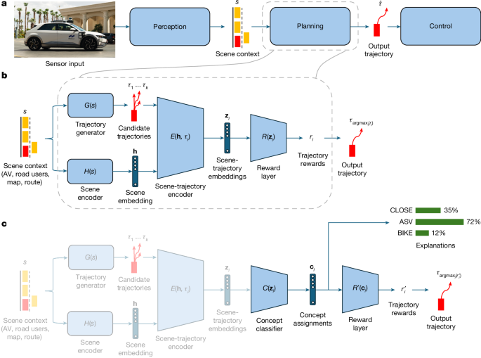
Architecture of the Interpretable Autonomous Driving Planner

The black-box machine-learning (ML) planner uses a modified DriveIRL architecture^1,2 (Fig. 1b). For the trajectory generator G, we use a heuristic generator that creates 143 jerk-optimal trajectories leading to anchor waypoints along the route. The scene encoder H is based on the hierarchical vector transformer (HiVT)⁵¹, pretrained for multi-agent motion prediction. In addition to generating the scene embedding h, HiVT produces three additional autonomous-vehicle (AV) trajectories, resulting in k = 146 candidate trajectories.

Within the scene–trajectory encoder E, each trajectory is encoded with a recurrent neural network. The trajectory representation is then combined with the scene embedding and processed by a transformer layer to generate scene–trajectory embeddings z_i. The reward model R is a multilayer perceptron (MLP). In CW-Net (Fig. 1c), both the classifier C and the new reward model \({R}^{{\prime} }\) are implemented as MLPs.

We did not evaluate additional methods beyond CW-Net because, at the time of writing, we were not aware of other approaches capable of modelling interpretable-by-design inverse reinforcement learning (IRL) systems. Our broader objective was to compare concept-based explanations, represented by CW-Net, with a no-explanation control condition. This comparison supports the generalizability of our findings across the wide range of concept-based explainable-AI techniques in the literature.

CW-Net Training for Explainable Autonomous Vehicles

We trained CW-Net using two datasets:

• Dataset 1: 500,000 driving scenarios with 8 concept labels (Supplementary Table 1).

• Dataset 2: 3,000,000 driving scenarios with 10 concept labels (Supplementary Table 2).

The complete list of concept labels and definitions appears in the section ‘Concept details’. Each scenario contained 146 candidate trajectories, producing between 73 million and 438 million training examples for the concept classifier. Each example could include multiple concept labels.

CW-Net training assumes access to the original dataset used to train the black-box ML planner, together with annotated, human-understandable concept labels for each data point. The annotations may be multi-label, allowing a single example to contain as many concepts as are relevant or useful. Models used for the CLOSE and ASV experiments were trained on dataset 1. Models used for the BIKE and PEDESTRIAN experiments were trained on dataset 2.

During training, the parameters of the trajectory generator G, scene encoder H and scene–trajectory encoder E remained frozen. Only the concept classifier C and the new reward model R′ were updated. Two loss functions were optimized jointly.

First, the concept classification loss \({{\mathcal{L}}}_{\mathrm{concept}}\) trains C to predict the correct concept labels. Depending on the semantics of each scenario type, this loss combines categorical cross-entropy and binary cross-entropy. For example, in dataset 1, categorical cross-entropy models the vehicle’s steering concepts (LEFT, RIGHT and STRAIGHT) and speed concepts (STOP and SLOW). Binary cross-entropy predicts whether other concepts are present, including ASV, INTERSECTION and CLOSE. These losses are averaged as follows:

Here, M_CCE denotes the number of concepts modelled with categorical cross-entropy, such as steering and speed. M_BCE denotes the number of concepts modelled with binary cross-entropy, such as the presence of ASV, INTERSECTION and CLOSE. The terms c_i,j and \({\widehat{c}}_{i,j}\) represent the true and predicted labels for the jth CCE concept at the ith data point. Similarly, c_i,l and \({\widehat{c}}_{i,l}\) represent the true and predicted labels for the lth BCE concept.

For dataset 2, we used binary cross-entropy for every concept, including the speed labels STOP, SLOW and FAST. In practice, these loss-function settings can be adjusted for the requirements of a particular autonomous-driving task.

Second, the trajectory loss \({{\mathcal{L}}}_{\mathrm{trajectory}}\) uses cross-entropy to train the network to select the correct trajectory. We define the correct trajectory as the trajectory originally selected by the black-box planner. The two losses are combined as follows:

We applied focal loss⁵² to address class imbalance, consistent with the original DriveIRL planner^1,2. The neural networks were trained computationally on a large distributed infrastructure using PyTorch Lightning.

Concept Separation and Explainable AI Performance

Post hoc interpretability modules can fail when the underlying network has not learned to distinguish the concepts of interest. In such cases, concept prediction accuracy may be limited⁵³. We observed this issue in an experimental prototype evaluated with supplementary table 2: concepts such as CLOSE and PEDESTRIAN showed relatively low precision but high recall.

Two considerations are important. First, more capable and better-trained architectures naturally learn to separate a substantial number of concepts in an unsupervised way^54,55,56. As a result, this limitation may become less significant as organizations develop larger flagship models.

Second, imperfect concept separation can itself provide a useful explanation. For example, if CW-Net cannot distinguish red traffic lights from green traffic lights, this may reveal why the AV fails to choose the appropriate action, such as stopping instead of proceeding. The underlying cause could be insufficient traffic-light examples in the training data. From an explainability perspective, concepts with lower accuracy can therefore be especially informative because they show where the model’s internal understanding is incomplete, as demonstrated in the paper.

Alternative Architecture for Post Hoc AV Explanations

In addition to the primary causal architecture shown in Fig. 1, we developed an alternative architecture that generates post hoc justifications for autonomous-vehicle behaviour (Extended Data Fig. 1). We froze the pretrained black-box ML planner and trained a concept-classifier head C in parallel with the reward layer R. As in the causal architecture (Fig. 1c), C classified concepts using the scene–trajectory embeddings z_i.

This parallel design is relatively simple and accessible. However, its explanations may be less faithful to the planner’s actual reasoning because the concept predictions do not directly influence how the model ranks state–trajectory pairs. Nevertheless, existing evidence indicates that post hoc explanations can be effective⁵⁷. We therefore include both architectures and demonstrate their practical value. The parallel architecture was used for real-world scenarios involving the CLOSE concept, described in the section ‘Unexpected stopping for nearby vehicles’.

Concept Definitions Used in CW-Net

Dataset 1 included the following concepts:

• LEFT, RIGHT, STRAIGHT: Driving-direction classifications trained with cross-entropy loss. For example, LEFT identifies scenarios in which the vehicle turned left.

• STOP, SLOW: Vehicle-speed classifications trained with cross-entropy loss. The STOP concept identifies scenarios in which the vehicle was stationary.

• ASV (approaching stopped vehicle): Scenarios in which the vehicle approached a stopped vehicle. This concept was trained with binary cross-entropy.

• INTERSECTION: Scenarios in which the vehicle was located at an intersection. This concept was trained with binary cross-entropy.

• CLOSE: Scenarios in which the vehicle was within 3 m of another vehicle. This concept was trained with binary cross-entropy.

Dataset 2 included the following concepts:

• SLOW: Scenarios in which the vehicle travelled at 1–2 m s⁻¹.

• STOP: Scenarios in which the vehicle was stationary.

• FAST: Scenarios in which the vehicle travelled faster than 2 m s⁻¹.

• STOP SIGN: Scenarios in which the vehicle was near a stop sign.

• TRAFFIC LIGHT: Scenarios in which the vehicle was near a traffic light.

• INTERSECTION: Scenarios in which the vehicle was at an intersection.

• PEDESTRIAN: Scenarios in which the vehicle was near a pedestrian.

• FOLLOWING: Scenarios in which the vehicle was following another vehicle.

• BIKE: Scenarios in which the vehicle was near a cyclist.

• PUDO (pedestrian pickup/drop-off): Scenarios in which the vehicle was in a pedestrian pickup–drop-off zone.

Every concept in dataset 2 was trained using binary cross-entropy.

Although the AV was trained on 8–10 concepts, depending on the dataset, our analysis focused on CLOSE, ASV, BIKE and PEDESTRIAN. These concepts relate directly to other road users and can be evaluated through counterfactual testing. FOLLOWING also involves other road users, but no notable examples occurred during real-world deployment.

Simulation Results for CW-Net Autonomous Driving

We evaluated CW-Net across the complete nuPlan validation dataset to compare its autonomous-driving performance with that of the original black-box ML planner. nuPlan is a large-scale autonomous-driving planning benchmark³⁹ that measures an AV’s similarity to human driving using L₂ distance, route progress and safety, measured by collision avoidance.

When following a lane or slowing from high speed, the black-box planner achieved more than 93% of the human driving distance, remained more than 90% collision-free and stayed within 1 m of the ground-truth human trajectory at 5 s. Performance decreased when the vehicle started from a stop: route progress fell to 74% of the human driving distance, collision-free performance fell to 81% and displacement from the human trajectory increased to 1.2 m at 5 s.

Across all measurements, our AV architecture differed from the original black-box agent by less than 0.01 L₂ on average. This difference was not meaningful, demonstrating that the more interpretable CW-Net architecture in Fig. 1 can be trained without sacrificing driving performance. Complete results are provided in Extended Data Table 1.

To verify concept accuracy, we evaluated 5% holdout data from both training datasets. Results are reported in Supplementary Tables 1 and 2. Across the two datasets, mean accuracy was 0.54, precision was 0.23, recall was 0.77 and the F1 score was 0.31. CW-Net did not separate every concept equally well. This outcome supports our explainability objective because the model’s explanations can reveal when concept separation fails and how those failures relate to driving performance, helping researchers refine their mental models.

Notable results included an F1 score of 0.82 for the SLOW concept and an F1 score close to zero for BIKE. The latter result suggests that the cyclist-related concept may not be well encoded or understood by the vehicle.

Mental Model Elicitation Studies for Explainable AVs

These studies replicated the driver experiences from the private-track tests described in the section ‘Mental model improvement in deployment’ using a larger participant group. The objective was to assess the robustness of findings concerning driver mental models (Extended Data Fig. 2). We conducted the study separately with experts, including drivers and test engineers from Motional, and non-experts recruited through Prolific.com.

We tested the following hypotheses:

• Hypothesis 1: Before viewing an explanation in the video replay, participant responses would more closely match the safety driver’s initial belief in the vehicle.

• Hypothesis 2: After viewing an explanation, participant responses would more closely match the safety driver’s updated belief.

• Hypothesis 3: After viewing an explanation, participant responses would more closely match the ground-truth reason for the AV’s behaviour.

• Hypothesis 4: Counterfactual prediction performance would correlate with the quality of a participant’s mental model, measured using nearest-neighbour tasks and free-form responses described in ref. ⁴³.

• Hypothesis 5: The two measures of mental-model quality would correlate and show similar distributions across participant groups.

Study Design and Materials

We examined the same three surprising events identified during the private-track tests. Mental models were measured using nearest-neighbour and prediction tasks, confidence ratings and free-form written explanations⁴³ (Extended Data Fig. 2).

Participants first watched each video and rated two possible explanations for the AV’s behaviour, including their confidence in each choice. This was the nearest-neighbour mental-model task. They then made the same counterfactual prediction as the driver, reported their confidence and provided a free-form rationale. Participants subsequently watched the video again with a CW-Net explanation and repeated the questions. This within-participant design reproduced the experience of safety drivers during on-road testing.

Participants

The expert group consisted of nine Motional safety drivers, test engineers and test specialists aged 18–80 years. Eight participants were male and one was female. All volunteered and received no payment.

The non-expert group consisted of 30 randomly selected US citizens recruited through Prolific.com (www.prolific.com). Participants were native English speakers aged 18–80 years, with an equal number of male and female participants. To support high-quality written responses, participants were paid USD15 per hour and were instructed to take part only if they fully understood the study instructions.

The study received approval from the MIT Institutional Review Board Committee on the Use of Humans as Experimental Subjects. The study was exempt under ID E-5903, with a start date of 1 July 2024 and an end date of 31 August 2026.

Mental Model and Prediction Metrics

We used the nearest-neighbour task and free-form written rationale as direct measures of mental models. For the nearest-neighbour task, mental-model quality combined choice accuracy and confidence. Improvement was defined as changing an incorrect belief to the correct ground-truth belief, increasing confidence in a correct belief or reducing confidence in an incorrect belief (Extended Data Fig. 3).

For the free-form rationale, an LLM-as-a-judge approach using GPT-5 determined which response—before or after viewing the CW-Net explanation—was closer to the ground-truth reason for the AV’s behaviour (see Supplementary Methods). Prompts were tuned over three iterations using expert responses (Extended Data Fig. 4a) and evaluated once on non-expert responses (Extended Data Fig. 4b). Improvement occurred when the post-explanation response was closer to the ground truth than the pre-explanation response.

We used the prediction task as an indirect measure of mental models because successful prediction depends on understanding the AV’s behaviour^44,58. Prediction improvement combined accuracy and confidence using the same approach as the nearest-neighbour task (Extended Data Fig. 5).

To assess the relationship between direct measures of mental models—nearest-neighbour scores and free-form rationales—and indirect prediction performance, we used a linear mixed-effects model (LME). The model tested whether mental-model changes, classified as improvement or worsening, affected the prediction-change variable, defined as the change in prediction confidence. Individual participant variation was included as a random effect (Extended Data Fig. 5).

To combine accuracy and confidence on one scale, confidence values for inaccurate beliefs were multiplied by −1. All analysis code will be made available upon publication (see section ‘Code availability’).

Mental Model Study Conclusions

The results supported all five hypotheses:

• Hypothesis 1: Before viewing the explanation, participant beliefs were often more similar to the safety driver’s initial belief (P < 10⁻⁹, exact binomial test).

• Hypothesis 2: After viewing the explanation, participant beliefs were more frequently similar to the safety driver’s final belief (P < 0.0002, exact binomial test).

• Hypothesis 3: Post-explanation beliefs were more often consistent with the ground truth (P < 10⁻⁵, exact binomial test).

• Hypothesis 4: Mental-model category was clearly related to predictive ability. The only non-significant relationship involved free-form text responses in the expert group (Extended Data Fig. 5).

• Hypothesis 5: Interaction analysis found no significant difference between expert and non-expert groups in the relationship between nearest-neighbour score improvement and rationale improvement (P = 0.842; Extended Data Fig. 4c). This result indicates a consistent underlying mechanism. Non-experts showed a significant positive correlation (β = 0.27, P < 0.001), meaning that improved nearest-neighbour scores strongly predicted improved written rationales. Experts showed a similar positive coefficient (β = 0.23), but the relationship was not statistically significant, probably because of the smaller sample size (P = 0.243).

Public-Road Evaluation Using SAGAT

We deployed CW-Net in manual mode on public roads in Las Vegas to collect complex, naturalistic scenarios similar to those identified during private-track testing (Extended Data Fig. 6). These scenarios formed the basis of an online Situation Awareness Global Assessment Technique (SAGAT) study involving 100 participants.

This approach enabled us to evaluate the robustness of CW-Net explanations using an established framework for measuring situational awareness (Extended Data Fig. 2). We used a between-participant design comparing CW-Net concept-based explanations with baseline explanations describing speed and steering⁴⁹ (Extended Data Fig. 7).

Collection of Public-Road Evaluation Materials

We collected data for ASV (01:02:55), CLOSE (00:50:42) and BIKE (more than 3 hours). We identified sequences in which human driving reproduced the ML planner’s behaviour in surprising situations resembling those from the private-track tests. Examples included CLOSE, in which the vehicle became stuck beside nearby vehicles, and ASV, in which it braked in response to hallucinated stopped vehicles (Extended Data Fig. 6).

Because no cyclists naturally appeared in the new video data, PEDESTRIAN replaced BIKE. We selected two surprising events for each concept, six events in total, together with six corresponding ‘unsurprising’ events. This ensured that the explanations did not reduce situational awareness during routine driving (Supplementary Table 5).

Activation thresholds were 0.5 for ASV/PEDESTRIAN and 0.94 for CLOSE. These thresholds were derived from earlier private-track data (Fig. 3).

The distribution of concept activations did not change significantly between private-track and public-road testing (Supplementary Table 7), even though the tests took place more than a year apart, used different AVs and software stacks, and occurred under substantially different conditions. This result supports the robustness and reliability of the CW-Net algorithm.

SAGAT Study Design

We conducted a between-participant SAGAT study (n = 100) measuring perception, comprehension and projection. Participants were assigned to either an experimental group that viewed CW-Net explanations or a control group that viewed speed and steering placeholders. Attention checks based on video content and viewing duration reduced the final sample to 99 participants: 51 in the experimental group and 48 in the control group.

SAGAT Study Materials

The study included 13 videos: six surprising events, six unsurprising events and one attention-check video. The experimental group viewed concept activations, while the control group viewed speed and steering information (Extended Data Fig. 8). After each video, a blackout screen displayed six binary questions: four assessing perception, one assessing comprehension and one assessing projection.

SAGAT Study Participants

We recruited gender-balanced US residents aged 18 years or older through Prolific.com. All participants were native English speakers and were paid $12 per hour. The study received MIT IRB approval from the Committee on the Use of Humans as Experimental Subjects. The study was exempt under ID E-5903, with a start date of 1 July 2024 and an end date of 31 August 2026.

Situational Awareness Metrics

For each participant, we calculated the average response for each question type. We used two-tailed t-tests and analysed surprising and unsurprising events separately across each dimension of situational awareness.

Public-Road Study Conclusions

After data collection and attention-check filtering, 99 of the intended 100 responses remained. Results are shown in Extended Data Fig. 7. During surprising events, CW-Net explanations significantly improved situational awareness after Bonferroni correction. The effects were large for perception (Cohen’s d = 1.290) and comprehension (d = 0.996), and medium for projection (d = 0.606).

During unsurprising events, no significant differences were observed: perception (d = 0.085), projection (d = −0.142) and comprehension (d = −0.514). These results indicate that concept-based explanations improve understanding in anomalous driving situations without reducing situational awareness during routine autonomous operation.

We also assessed feature robustness by comparing concept distributions with earlier private-track tests using Wasserstein distance (Supplementary Table 7). The analysis found no meaningful distribution changes.

Reporting Summary

Additional information about the research design, participants, methods and analyses is available in the Nature Portfolio Reporting Summary linked to this article.