


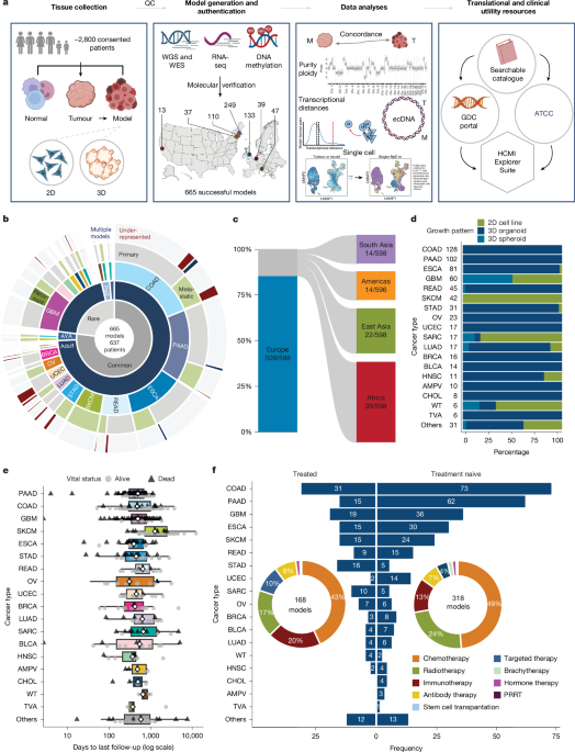
Biospecimen processing and quality control
Before nucleic acid extraction, all frozen and formalin-fixed, paraffin-embedded (FFPE) tumour and normal specimens underwent pathology quality control (QC). For frozen tissue, a piece measuring up to 30 mg was prepared. For FFPE tissue, an equivalent number of scrolls was cut from the block. Haematoxylin-and-eosin-stained sections from the top and bottom of each specimen were scanned and reviewed by a pathologist to confirm the reported tumour histology and estimate tumour cellularity, necrosis and other pathological features. Average tumour nuclei and necrosis percentages were calculated from both slides. Tumour samples were eligible for nucleic acid extraction when they contained at least 50% tumour nuclei and no more than 20% necrosis. Normal tissues were excluded if any tumour cells were detected.
DNA was extracted from normal blood and saliva. DNA and RNA were co-extracted from tumours, solid normal tissues and cancer models. Cancer models were washed with ice-cold PBS before extraction to remove residual Matrigel. Frozen tissues and models were homogenized with a Qiagen TissueLyser, followed by DNA and RNA extraction using a modified Qiagen DNA/RNA AllPrep workflow. The homogenate was applied to a Qiagen DNA column, and the flow-through was processed with the mirVana miRNA Isolation kit (Ambion). FFPE samples were deparaffinized and lysed. DNA was extracted from the pellet using the AllPrep FFPE kit (Qiagen), while RNA was isolated from the supernatant using the Highpure miRNA kit (Roche). Blood DNA was extracted with the QiaAmp DNA Blood Midi kit (Qiagen), and saliva DNA with the Gentra Puregene Buccal Cell kit (Qiagen).
DNA concentration was measured with a PicoGreen assay, while RNA concentration was determined by absorbance at 260 nm using a UV spectrophotometer. DNA integrity was assessed by 1% agarose gel electrophoresis to confirm the presence of high-molecular-weight fragments. RNA quality was measured with the RNA6000 Nano assay on an Agilent Bioanalyzer. RNA from frozen tissues was assigned an RNA integrity number (RIN), whereas FFPE RNA was evaluated using the DV200 metric. All DNA samples underwent genotyping with a custom Sequenom single-nucleotide polymorphism (SNP) panel or AmpFISTR Identifiler (Applied Biosystems) to confirm that specimens from the same case originated from the same patient.
Genome sequencing
Whole-genome sequencing data processing
Whole-genome sequencing (WGS) reads were processed with the Genomics Data Commons (GDC) DNA-seq alignment pipeline59 and mapped to a customized GRCh38 reference genome. Reads were aligned with BWA-MEM (v.0.7.15)60, then sorted, merged and marked for duplicates with Picard Tools (v2.26.10). Base-quality scores were recalibrated using GATK (v.3.7.0)58 and base-quality score recalibration. Sample contamination was estimated with GATK ContEst. Samples with contamination levels above 4% were excluded from downstream analysis.
SNV and indel variant calling
New York Genome Center pipeline. The NYGC v.6 somatic SNV and indel pipeline61 was applied to each tumour–normal and model–normal pair using GDC-aligned BAM files. SNVs, multi-nucleotide variants (MNVs) and indels were identified with MuTect2 (GATK v.4.0.5.1)62, Strelka2 (v.2.9.3)63 and Lancet (v.1.0.7)64. SvABA (v.0.2.12)65 was also used for indel detection, and Manta (v.1.4.0)66 candidate indels were supplied to Strelka2 according to the developer’s recommendations.
Variant calls were merged and annotated with Variant Effect Predictor (v.93.2)75 and Ensembl (v.93)67, COSMIC (v.86)47, 1000Genomes Phase 368, ClinVar69, PolyPhen70, SIFT71, FATHMM72, gnomAD73 and dbSNP74. Variants were filtered when they occurred in at least two normal samples, had a population minor allele frequency of at least 1%, tumour variant allele frequency (VAF) below 0.0001, normal VAF above 0.2, sequencing depth below 2× in either sample, or higher VAF in the normal than the tumour sample. The panel of normal samples contained 242 unrelated individuals sequenced across Illumina HiSeqX and NovaSeq platforms at the NYGC and through the Illumina Polaris project.
Broad whole-exome sequencing pipeline. Whole-exome sequencing (WES) BAM files underwent the same alignment and quality-control workflow. SNVs were called with MuTect and small indels with Strelka. Tumour-in-normal contamination was estimated with deTiN, while cross-participant contamination was assessed with ContEst. WES and WGS variants were processed using previously described methods77.
WashU pipeline. The TinDaisy2 somatic variant pipeline (v.2.6.2; https://github.com/ding-lab/TinDaisy) was used for WGS and WES SNV and indel calling. Tumour and normal BAM files were analysed with VarScan (v.2.3.8)79, Strelka2 (v.2.9.10)63, Pindel80 and MuTect (v.mutect-1.1.7)81. Calls were retained when their length was below 100 bp, normal VAF was no more than 0.02, tumour VAF was at least 0.05, tumour depth exceeded 14×, normal depth exceeded 8× and at least two callers supported the variant. Variants were annotated with VEP 9982, filtered by population allele frequency and normalized with bcftools (v.1.10.2)84.
Consensus variant calling. The MergeParticipantVcfs workflow combined pair-level VCF and MAF files from the NYGC, Broad and WashU pipelines. Multi-allelic variants were split, MNVs were labelled and normalized, centre-specific annotations were retained, and indels were left-aligned. Prepared files were merged with BCFTools84. Allele depth, read depth and allele frequency were recalculated from BAM pileups using a custom method61, and MNVs were re-established. MuTect2 force calling was then performed on the multisample VCF, followed by filtering using read-orientation metrics.
Final calls were annotated with Ensembl VEP, COSMIC, 1000Genomes, ClinVar, PolyPhen2, SIFT, FATHMM, gnomAD and dbSNP. High-confidence VCFs were generated with the MakePairHighConfidenceVcfs workflow. Calls were removed when MuTect2 failed them and were added when read support was present in all non-normal WGS BAM files from the same participant, even if a formal call was not made for an individual pair.
Copy number calling
ASCAT method. Tumour purity and ploidy were estimated for each tumour–normal and model–normal pair using AscatNGS (v.4.2.1)85 with default parameters.
ABSOLUTE method. Copy number segmentation was performed with fragcounter, ReCapSeg and AllelicCapSeg. AllelicCapSeg results were supplied to ABSOLUTE together with WES or WGS mutation calls to infer allelic integer copy numbers. ABSOLUTE solutions were manually curated, and the solution that best matched the observed copy number profile was selected. For samples without copy-number alterations, the optimal solution was inferred from SNV multiplicity.
ReMixT method. ReMixT86 was applied to WGS data to estimate allele-specific and clone-specific copy numbers using established methods87.
PURPLE method. B-allele frequencies were generated with AMBER, and read-depth ratios were calculated with COBALT88. These results were integrated with somatic SNVs and structural variants to estimate tumour purity, ploidy and copy-number profiles with PURPLE. Samples without matched normal tissue were processed using updated AMBER, COBALT and PURPLE versions. The tools are freely available from the Hartwig Medical Foundation (https://github.com/hartwigmedical/hmftools).
HATCHet method. HATCHet-289 was used to estimate purity, ploidy and clonal copy numbers. Default parameters were applied with predefined hidden-Markov-model state and transition settings, a diploid B-allele-frequency threshold of 0.06, a maximum neutral shift of 0.06 and a two-to-four-clone search space. Gurobi was used as the preferred integer-linear-programming optimizer.
Consensus copy-number method. The ABSOLUTE solution closest to the consensus purity and ploidy estimates was selected for each sample. Where ABSOLUTE and consensus estimates differed, the consensus solution was retained unless manual review indicated that it poorly represented the underlying copy-number states. ABSOLUTE force calling was then used to generate segmented allelic copy-number states across the genome.
Structural variant calling
NYGC pipeline. Somatic structural variants (SVs) were identified from GDC-aligned BAM files using SvABA, Manta and Lumpy61,65,66,90. SVs shorter than 500 bp were excluded. Remaining calls were merged with bedtools using a 300 bp slop, matching strand orientation and at least 50% reciprocal overlap. SVs were annotated against 1000Genomes, DGV, gnomAD-SV and a panel of normal samples. Variants overlapping these resources were removed from the final callset.
Broad pipeline. SVs were called with Manta, SvABA and dRanger. Breakpointer was used to refine breakpoint locations. An event had to be detected by at least two callers within a 350 bp clustering window and pass filters based on genomic span, mapping quality and supporting reads.
WashU pipeline. Manta (v.1.6.0)66 was applied to matched tumour–normal WGS data. Calls were filtered using site depth, somatic score and MAPQ0 read-fraction criteria, then converted to BEDPE format with svtools (v.0.5.1)95 (https://github.com/hall-lab/svtools).
MSKCC pipeline. SVs were identified with deStruct and LUMPY, retaining only shared breakpoints. Filters excluded poorly supported events, deletions below 1,000 bp, breakpoints with fewer than five tumour-supporting reads and events with any support in the matched normal sample.
EMBL-EBI pipeline. Somatic SVs were called with GRIDSS2, annotated using RepeatMasker and kraken2, and filtered with GRIPSS. The final SV set was refined with PURPLE copy-number profiles and visualized with ReConPlot. Unmatched samples were analysed with updated GRIPSS and PURPLE versions.
Consensus SV method. Consensus SVs from the NYGC, Broad, WashU, MSKCC and EMBL-EBI pipelines were identified with a modified bedtools pair2pair workflow102. Multicaller consensus files from each centre were merged using a 50 bp slop value. SVs detected by at least two analysis centres were accepted into the final consensus set.
Tumour purity and ploidy
ESTIMATE. Tumour purity was inferred from gene-expression data using the ESTIMATE algorithm103, which measures stromal and immune gene signatures. Purity was calculated as follows: tumour purity = cos (0.6049872018 + 0.0001467884 × ESTIMATE score).
Consensus purity and ploidy. Consensus purity and ploidy were derived from five DNA-based callers—ASCAT, ABSOLUTE, ReMixT, PURPLE and HATCHet—and the RNA-based ESTIMATE method. The mean purity was calculated iteratively. Values within ±0.2 of the mean were accepted; outlying callers were removed one at a time until the remaining estimates converged or fewer than three callers remained. In the latter case, ABSOLUTE was preferred, followed by PURPLE when ABSOLUTE was unavailable.
Ploidy estimates were grouped into haploid, diploid, triploid and tetraploid classes. When at least three callers agreed on a class, the median value within that class was used. Otherwise, ABSOLUTE or PURPLE was selected. All consensus values underwent manual review, and the ABSOLUTE solution was retained when the consensus estimates did not accurately reflect the underlying copy-number profile.
Genomic analysis methods
Tumour–model SNV concordance. Variants were included when their VAF exceeded 0.15 or when all non-normal aliquots contained supporting reads.
Tumour–model loss-of-heterozygosity concordance. Loss of heterozygosity (LOH) was defined when the rounded minor copy number for a genomic bin equalled zero. LOH status was compared between each tumour and its matched model, with concordant and discordant bins scored as 1 and 0, respectively. The mean across equal-sized genomic bins provided one LOH concordance score per pair.
Whole-genome duplication. Whole-genome duplication (WGD) status was inferred from genome-wide copy-number alterations. The fraction of the genome affected by copy-number gains was calculated after weighting each segment by genomic length. Samples with gains across most of the genome above the predefined threshold were classified as having one WGD event; samples exceeding the higher threshold were assigned multiple WGD events.
Mutation signatures. Single-nucleotide variant mutational signatures were calculated with the GPU version of SignatureAnalyzer104,105 using COSMIC single-base substitution references. Fifty-one non-redundant signatures were selected, and each tumour and matched model was represented by a signature exposure profile. Tumour–model similarity was measured using cosine similarity and compared with randomized pairs from the same or different cancer types.
Driver gene classification. Driver genes were curated from TCGA studies106. SNV, indel and copy-number results were integrated. Only moderate- or high-impact variants were analysed, together with TERT promoter mutations. Gene-level copy numbers were calculated across each gene. High-level amplification required a ploidy of at least 1.5 and either a copy number of at least 3 and twice the ploidy, or a copy number of at least 7. Homozygous deletion was defined as a copy number below 0.3.
For visualization, shared tumour–model mutations were classified as gain-of-function (GOF) or loss-of-function (LOF). LOF events included homozygous deletions, frameshift variants, nonsense mutations and splice-site alterations. GOF events included missense mutations, high-level amplifications, TERT promoter mutations and in-frame indels. A gene was classified as LOF when more than 15% of shared mutations were LOF; otherwise, it was classified as GOF. Genes without shared mutations were labelled unclassified.
Power calculation. The power to detect model-derived SNVs in tumours was estimated assuming that each mutation was clonal and present on one allele. The expected variant allele frequency at a genomic position with tumour copy number T was calculated as
$$\mathrm{VAF}=\frac{\rho }{\rho T+(1-\rho )N}$$
Here, N represents the copy number in contaminating cells and was assumed to be two for autosomes. Assuming a binomial distribution and that one alternative read was sufficient for detection, average detection power was calculated as
$$\mathrm{Power}\,\mathrm{to}\,\mathrm{detect}=\frac{1}{N}{\sum }_{i}^{N}1-{\mathrm{Binom}}_{\mathrm{CDF}}({C}_{i},0,{\mathrm{VAF}}_{i})$$
Here, BinomialCDF is the binomial cumulative distribution function, Ci is tumour read coverage at the ith model SNV and N is the number of autosomal SNVs evaluated.
ecDNA analysis. Raw coverage was calculated from GDC-aligned BAM files with fragCounter and corrected with dryClean using a panel of 390 normal samples. CBS was then used to calculate tumour–normal coverage ratios and segment the genome. Consensus purity, ploidy and SV profiles were integrated with JaBbA to construct junction-balanced genome graphs. AmpliconSuite-pipeline, AmpliconArchitect and AmpliconClassifier were used to detect and classify amplified DNA structures, including extrachromosomal DNA (ecDNA).
Paired tumour–model amplicons were considered concordant when they received the same classification and had a Jaccard genomic interval similarity of at least 0.75. Putative cyclic ecDNA structures were reconstructed with Candidate Amplicon Path EnumeratoR and visualized with CycleViz (https://github.com/AmpliconSuite/CycleViz).
Clonal phylogenies. Force-called SNVs and consensus copy-number states were analysed with pyclone-vi and phyclone. Indels were excluded. Pyclone-vi used a beta-binomial model, 10 restarts and up to 40 clusters. Clusters containing fewer than 1% of SNVs or approximately 0.5 cancer-cell fraction across all samples were removed. The remaining clusters were analysed with phyclone using 16 chains, 100,000 iterations and an outlier probability of 0.1.
Genetic ancestry estimation. Genetic ancestry proportions were estimated with ADMIXTURE123,124 using reference markers from 1,964 unrelated 1000Genomes samples. Germline markers were genotyped from WGS data with GATK pileup. Admixed reference populations were excluded, and markers were filtered by minor allele frequency and linkage disequilibrium using PLINK. Each sample was assigned proportions across five continental populations and 23 reference populations, then categorized according to its largest continental ancestry component.
DNA methylation and epigenetic fidelity
DNA methylation data processing
DNA methylation was profiled with the Illumina HumanMethylationEPIC v1 array. Raw IDAT files generated on the Illumina iScan system were downloaded from the GDC data portal (https://portal.gdc.cancer.gov). Methylation beta values were calculated with the openSesame pipeline in SeSAMe (v.1.18.4)125.
Normal tissue methylation and probe selection
Normal-tissue methylation profiles were used to identify cancer-associated DNA hypermethylation. Previously identified CpGs that were unmethylated across eight normal tissues were combined with ENCODE gastrointestinal tissue data. EPICv1 IDAT files from 23 gastrointestinal samples were processed using openSesame. The final analysis used 144,571 CpGs that were unmethylated in normal tissues across 12 tissue types.
TCGA and TARGET DNA methylation data
TCGA Pan-Cancer Atlas methylation data generated with the Infinium HumanMethylation450 array were downloaded and processed with SeSAMe. TARGET neuroblastoma and Wilms tumour IDAT files were obtained from the GDC portal and processed using the same workflow. The analysis included 130 Wilms tumours and 91 adrenal neuroblastomas.
Joint HCMI and TCGA–TARGET methylation dataset
HCMI EPICv1 and TCGA–TARGET HM450 data were merged using probes shared between the platforms125. Samples with probe success rates below 90% were excluded, as were probes with more than 10% missing values and probes on the X and Y chromosomes. Among CpGs normally unmethylated in tissue, 53,204 sites acquired methylation with a beta value above 0.3 in at least two HCMI cancer samples.
UMAP analysis of DNA methylation profiles
Non-negative matrix factorization (NMF) was used to reduce the combined HCMI and TCGA–TARGET methylation matrix. Zero beta values were replaced with 1.0 × 10⁻¹², and missing values were set to zero. Models with ranks from 2 to 200 were evaluated with three random starts. Rank 170 produced the lowest and most consistent reconstruction error. UMAP visualization was generated from the rank-170 NMF representation using cosine distance.
DNA methylation heatmap
For four cancer cohorts, the 10% most variable CpGs were identified separately and combined into a set of 8,614 sites. Beta values were converted into binary methylation calls using a threshold of 0.3. Sample distances were calculated with the Jaccard index, followed by unsupervised hierarchical clustering. Heatmaps were generated with ComplexHeatmap (v.2.20.0)131.
Tumour–model DNA hypermethylation similarity
DNA methylation similarity between each model and its parental tumour was assessed using cancer-associated CpG hypermethylation profiles. Pearson correlation coefficients were calculated for matched model–tumour pairs, unmatched samples from the same cancer type and unmatched samples from different cancer types. After false-discovery-rate correction, pairs with adjusted P ≥ 0.1 were considered non-concordant.
Transcriptional fidelity and relatedness
RNA processing and sequencing
RNA quality control. RNA from fresh-frozen models and FFPE tumours was assessed for concentration, integrity and fragment size. Fresh-frozen RNA was evaluated with RIN, with values above 8.0 considered high quality. FFPE RNA was assessed using DV200 and fragment-size measurements.
Total RNA-seq library preparation. Libraries were prepared with the Illumina Stranded Total RNA Prep with RiboZero Gold kit and individually barcoded. Samples were pooled using automated liquid handling, with typical pools containing 38–92 libraries. Library concentration, size and distribution were evaluated with a TapeStation system. MiSeq Nano sequencing was used when additional pool or library QC was required.
Total RNA sequencing. Indexed libraries were sequenced on an Illumina NovaSeq 6000 using paired-end 100 bp reads. Each library targeted at least 150 million reads and more than 90% mapped reads. Reads were demultiplexed and converted to FASTQ files, followed by adapter and low-quality sequence assessment. Samples were evaluated by mapping to hg38, measuring coding-region alignment, rRNA content, gene detection and housekeeping-gene expression. Passing samples were clustered with related tumour types to confirm expected expression patterns. Atypical samples were SNP-typed to verify specimen identity, and FASTQ files were deposited in the GDC repository.
MicroRNA sequencing. Small-RNA libraries were prepared with the NEXTflex Small RNA-seq kit v4, individually barcoded and processed on a Sciclone liquid-handling workstation. Library concentration and fragment distribution were assessed with TapeStation and Bioanalyzer instruments. Libraries were size-selected before sequencing, and post-sequencing QC evaluated miRNA abundance and diversity.
Transcriptional relatedness analysis
MOMA subtype identification. Tumour subtypes were compared with TCGA MOMA subtypes using OncoMatch38. MOMA identifies transcriptional cell states through the activity of master regulators, including transcription factors and co-factors. VIPER estimated regulator activity from target-gene expression, while ARACNe inferred regulatory networks. Samples were clustered according to regulator activity using partitioning around medoids.
MOMA subtype comparison. MetaVIPER was used to estimate transcription-factor and co-factor activity across HCMI samples. The top 50 differentially active regulators in each sample were compared with regulator signatures from 112 TCGA MOMA subtypes. OncoMatch scores integrated enrichment in both directions using Stouffer’s method. When a matched tumour and model shared a significant subtype assignment, the subtype with the strongest integrated score was selected.
MetaVIPER and regulatory networks. MetaVIPER integrated VIPER statistics across lineage-matched networks. NaRnEA replaced the original aREA gene-set method to improve significance estimation. ARACNe3 networks were generated from 32 TCGA cancer cohorts and pruned to the 100 most significant targets for each regulatory protein. Networks included 1,645 transcription factors and 1,556 co-factors.
Differential expression signatures. TPM-normalized expression data were processed with the scGEN variational autoencoder to reduce batch effects. For each sample, expression was centered by the cohort median and scaled by the median absolute deviation. Protein-coding gene expression profiles were downloaded from the GDC portal and used to generate VIPER signatures.
Tumour–model similarity. Tumour and model expression profiles were normalized separately to prevent sample-type batch effects. MetaVIPER and cancer-type-specific regulatory networks were used to estimate protein activity. For small or rare cohorts, lineage-matched networks were combined and the most informative networks were retained. A nonparametric null distribution was generated from unrelated model–tumour comparisons, and matched pairs with FDR > 0.1 were considered poor transcriptional matches.
Celligner. Celligner was used to integrate HCMI tumours and models with TCGA, TARGET and CCLE expression data31. Contrastive principal component analysis identified immune, stromal and other non-malignant signals that could distort tumour–model comparisons. These components were removed before mutual-nearest-neighbour batch correction. The integrated data were subjected to PCA, and Euclidean distances were calculated in 70-dimensional principal-component space. Matched pairs with adjusted P ≥ 0.1 were classified as non-concordant.
Celligner input data. TARGET, TCGA and CCLE expression profiles were obtained from Xena and DepMap resources. HCMI TPM data were downloaded from the GDC portal. Expression values were log2 transformed after adding a pseudocount of 1 and restricted to 18,550 protein-coding genes shared across all datasets.
Euclidean and latent transcription-factor distances. Cancer cohorts and specimen types were analysed independently. Gene expression was restricted to biologically relevant, feature-selected genes. Euclidean distances were calculated as the mean pairwise distance across genes, and outliers were defined as values above 3 standard deviations. Latent transcription-factor distances were derived from a variational autoencoder trained on TCGA and GTEx normal tissues, with distances calculated in the resulting latent space.
Multiclass pair-classification distances. Relative expression of gene pairs was used to reduce batch effects and classify samples against TCGA-derived subtypes. Assignment-probability distances were calculated for matched HCMI tumour–model pairs. Distances above the third quartile plus 1.5 times the interquartile range were classified as outliers.
Canonical parallel direction. Expression matrices were transformed with the DESeq2 variance-stabilizing transform. Differences between matched tumour and model profiles were subjected to PCA, and the first loading vector defined the canonical parallel direction. Pairwise distances were calculated by projecting samples onto this direction. Values more than two standard deviations from the mean were considered outliers.
HCMI and CCLE model coverage comparison
To evaluate how effectively cancer models represent primary tumours, we measured the proportion of TCGA tumours with at least one high-fidelity model in HCMI, CCLE or the combined repository. High-fidelity models were defined by an OncoMatch normalized enrichment score of at least 1038,39. Violin plots showed the highest OncoMatch score available for each tumour across the model collections. Batch-corrected TPM expression data were processed with scGEN, and MetaVIPER estimated transcription-factor and co-factor activity using TCGA-derived ARACNe networks.
Tumour molecular pathology subtype prediction
Each sample was classified with tumour molecular pathology (TMP) models trained on TCGA primary tumours using gene expression, copy-number variation, DNA methylation, miRNA expression and somatic mutation data32. Because of their strongest performance, models based on gene expression or DNA methylation were applied to HCMI samples. Gene-expression data were quantile ranked before classification. A single subtype was reported for each sample based on the consensus of model predictions and confidence scores.
Single-nucleus RNA sequencing analysis
snRNA-seq sample preparation and analysis
Frozen samples from 17 tumour–model pairs were processed with the Chromium Nuclei Isolation kit and RNase inhibitor. Tissue was homogenized, filtered and centrifuged to remove debris. Isolated nuclei were loaded onto the 10x Genomics Chromium platform for gel-bead-in-emulsion generation, barcoding, reverse transcription and cDNA amplification. Libraries were prepared with the Chromium Single Cell 3′ Gene Expression protocol and sequenced on a NovaSeq instrument.
Short reads from 34 samples were aligned to the GRCh38-2024-A human reference genome with Cell Ranger (v.8.0.1)152. Base-call files were converted to FASTQ format with cellranger mkfastq, and gene-expression matrices were generated with cellranger count. Cell Ranger applied default QC filters and produced UMI count matrices for downstream analysis.
snRNA-seq demultiplexing
Samples sharing a 10x Chromium flow cell were demultiplexed with Demuxlet153. Germline variants were called from matched normal WGS data and filtered using gnomADv4 exome data. Only biallelic SNPs with a population MAF of at least 0.1%, presence in gnomADv4 and PASS status were retained. Cells were assigned to samples using Demuxlet. Doublets, ambiguous droplets and barcodes with a doublet probability above 0.99 were excluded from downstream analysis.
snRNA-seq gene-expression analysis
Demultiplexed UMI matrices were analysed with Scanpy (v.1.9.3)156. Cells were retained when mitochondrial RNA represented less than 25% of transcripts and UMI counts ranged from 800 to 50,000. Adjusted thresholds were used for selected low-cell-count samples. One tumour–model pair was excluded because of insufficient cell numbers, leaving 16 pairs for analysis.
UMI counts were normalized, log transformed and scaled. PCA, nearest-neighbour graphs and UMAP embeddings were generated with Scanpy. Leiden clustering was optimized by testing resolutions from 0.01 to 1.01 and selecting the solution with the highest mean silhouette score.
Copy-number analysis and malignant-cell detection
Copy-number alterations were inferred from single-nucleus expression data with inferCNV157. Reference nuclei were selected from non-malignant cell types in GBM, pancreatic adenocarcinoma (PAAD) and colorectal adenocarcinoma (COAD) samples. Cell identities were assigned using marker-gene over-representation analysis and publicly available PanglaoDB references. InferCNV was run with predefined filtering, hidden-Markov-model, denoising and subclustering parameters. Nuclei were labelled malignant when their inferred copy-number profile matched alterations detected by WGS in the corresponding bulk sample.
Cell-type annotation in GBM samples
GBM nuclei were assigned broad cell types using over-representation analysis with canonical brain markers. To improve signal-to-noise ratios, UMI counts were softly imputed by summing the counts of the 10 nearest neighbours. Nuclei not assigned as oligodendrocytes or microglia but located in putative malignant clusters were classified as malignant.
Malignant-state assignment in GBM
For each malignant GBM nucleus, a standardized gene-expression signature was calculated as follows: \({z}_{i}^{(k)}=\frac{{x}_{i}^{(k)}-{\overline{x}}_{\mathrm{ref}}}{{\sigma }_{\mathrm{ref}}}\). Signatures were evaluated against six established GBM cellular states—NPC1-like, NPC2-like, MES1-like, MES2-like, AC-like and OPC-like—using NaRnEA through pyVIPER. Each nucleus was assigned to the state with the highest normalized enrichment score. Nuclei with a minimum P value above 0.15 were labelled unknown. NPC1-like and NPC2-like states were combined as NPC-like, and MES1-like and MES2-like states were combined as MES-like.
Cell-type annotation in PAAD and COAD
PAAD and COAD nuclei were annotated with the Python implementation of SingleR using the Blueprint-ENCODE reference161,162. Soft gene imputation was performed by adding UMI counts from the 10 nearest neighbours before annotation. Epithelial nuclei within inferCNV-defined malignant clusters were labelled malignant. A small group of COAD nuclei annotated as neurons was also retained because of their likely neuroendocrine malignant phenotype.
Malignant-state assignment in PAAD
PAAD malignant nuclei were classified using published bulk and single-cell subtype frameworks. Protein activity was estimated with MetaVIPER using six PAAD regulatory networks derived from single-cell, laser-microdissected, TCGA, ICGC, UNC and HCMI data. Nuclei were assigned to the GLS, MOS or PLS transcriptional lineage according to the highest NaRnEA enrichment score. Cells with a highest-scoring subtype P > 0.15 were labelled unknown.
Malignant-state assignment in COAD
COAD malignant nuclei were evaluated against the iCMS2 and iCMS3 intrinsic subtypes using NaRnEA. Each nucleus was assigned to the subtype with the highest normalized enrichment score, while nuclei with P > 0.15 were classified as unknown. The analysis showed that tumour-derived models retained both major cellular states observed in the parental tumours, although their relative proportions varied.
Tumour–model differential gene expression
Differential gene expression between matched tumours and models was assessed with Scanpy after log transformation. The Wilcoxon rank-sum test and Benjamini–Hochberg correction were used to identify significant genes. Resulting signatures were analysed for pathway enrichment using pyVIPER and appropriate MSigDB, GBM meta-module and bulk transcriptional gene sets.
Medium-switching assay
To evaluate culture-medium effects on transcriptional plasticity, HCM-BROD-0416-C71 GBM cells maintained in NSA medium were transferred to formulated-conditioned medium. After recovery and expansion, cells were plated on laminin-coated vessels and switched to the new medium after 24 h. Cells were cultured for 72 h or 2 weeks, fixed, stained for the indicated markers and imaged with an Operetta CLS High-Content Analysis system. Additional experimental details are provided in the Supplementary Methods.
In vitro drug-sensitivity testing
Patient-derived GBM cells were maintained in NSA medium supplemented with epidermal growth factor and fibroblast growth factor. Cells were seeded at 2,000 cells per well in ultra-low-attachment 96-well plates. After 24 h, temozolomide was added using a D300e digital dispenser in an eight-point concentration series ranging from 0.03 to 300 µM. Cell viability was measured after 5 days with the CellTiter-Glo luminescent assay.
HCMI Explorer Suite
The HCMI Explorer Suite is a web-based R Shiny application developed to support exploration of HCMI genomic, clinical and translational data. Built with R Shiny (v.1.8.1.1)171 and R (v.4.3.2), the platform enables users to investigate treatment timelines, model-specific genomic profiles and transcriptional similarities among cancer models, matched tumours, TCGA samples and CCLE cell lines. Visualizations were created with ggplot2 and plotly, while the Clinical Module uses swimplot to display treatment histories and model exposures.
The application is deployed through Shiny Server, with analysis performed server-side. Source code is available on GitHub (https://github.com/human-cancer-model-initiative/HCMI-Explorer-Suite), and the hosted application is available at https://appshare.cancer.gov/HCMI_Explorer_Suite/.
Ethics statement
Human tissue samples and associated clinical information were collected through the Human Cancer Model Initiative (HCMI) under protocols approved by the Institutional Review Boards of participating Cancer Model Development Centres and clinical sites. All procedures complied with applicable ethical standards, regulations and HCMI requirements. Written informed consent was obtained from every participant before sample collection. Participating centres completed all required regulatory procedures, including institutional approval, consent documentation and data-sharing agreements.
Reporting summary
Additional information about the study design, experimental procedures and reporting standards is available in the Nature Portfolio Reporting Summary linked to this article.
Source: www.nature.com