


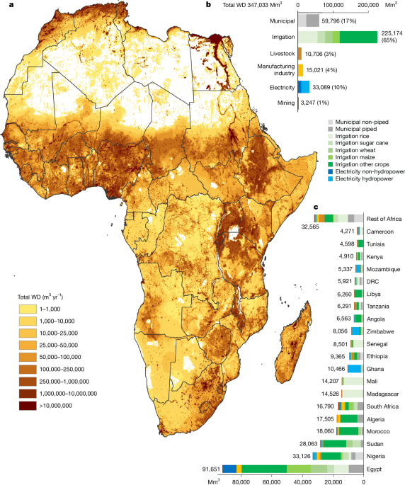
This assessment estimates sectoral and subsectoral water demand (WD) across mainland Africa and Madagascar for 2010 and 2020, covering municipal water, irrigation, livestock, manufacturing, electricity generation and mining. It combines measured utility data, international databases, modelling and geographic information system (GIS) analysis to produce estimates at spatial resolutions as fine as 2.5 arcminutes—about 4.5 kilometres at the equator. Because measured water-use data are scarce, particularly across Africa, the results are best estimates and include analyses of uncertainty around irrigation efficiency, municipal losses, environmental flows and mine production.
Scope and definitions
The study estimates the water demand of six sectors and their subsectors: municipal water, irrigation, livestock, manufacturing, electricity production and mining, for 2020 and 2010.
WD is the volume of water a sector would use to meet its needs if sufficient water were available1,2,8. When water is insufficient, the need is not fully met, which can reduce the performance of an activity. During a dry period, for example, farmers may be unable to irrigate all their crops, reducing yields. Similarly, a person without nearby drinking-water infrastructure may have to collect water from a distant source and consequently lack enough water for activities such as washing or cleaning. This assessment quantifies the water demand required to satisfy all sectoral needs.
The study measures water withdrawal (WW), not water consumption (WC)10. WW, also called water abstraction, is the volume withdrawn from rivers, lakes or aquifers. WC is the portion of that withdrawal that is not returned to the original source, for example because it evaporates. The difference between WW and WC is return flow. The term “water use” can refer generally to either WW or WC, so the distinction is important.
Most sectors were calculated at a resolution of 5 arcminutes, representing 371,665 data points. Municipal and industrial WD were calculated at 2.5 arcminutes. A 2.5-arcminute cell is 0.041667 degrees, or about 4.5 kilometres at the equator; a 5-arcminute cell is 0.08333 degrees, or about 9 kilometres at the equator. Within a 0.5-degree cell—the resolution used by many existing studies—the analysis contains 144 cells at 2.5 arcminutes and 36 cells at 5 arcminutes.
Mining and electricity data are represented as point data, the most detailed spatial resolution possible. Total WD, which combines all six sectors, is limited to 5 arcminutes because the underlying SPAM crop data13 and Gridded Livestock of the World (GLW) data48,49 are available at that resolution. No crop- or livestock-specific spatial datasets covering Africa are available at a higher resolution, making 5 arcminutes the highest feasible resolution for total WD.
Africa’s population was 1.36 billion in 2020 and 1.05 billion in 2010, an increase of 30%. The analysis covers mainland Africa and Madagascar, comprising 49 countries, with Morocco including Western Sahara. It excludes Cabo Verde, Comoros, Mauritius, Mayotte, Réunion, Saint Helena, Ascension and Tris, São Tomé and Príncipe, and Seychelles.
The assessment is based on extensive data mining, modelling and GIS analysis. Supplementary Table 1 lists the main data sources, while Supplementary Table 2 contains additional sources. The general workflow is shown in Extended Data Fig. 2. The overall method is a bottom-up approach.
Maps were created with ArcGIS using country and administrative borders from the Global Administrative Areas (GADM) database50. Figures use the Equal Earth projection51, which is endorsed by the African Union52 and recommended in a United Nations resolution passed by vote on 4 September 2026 (ref.53).
Why measured water-use data are scarce
Sectoral water use is difficult to quantify because the most accurate approach is to measure physical withdrawals directly. In the domestic sector, this can be done with water meters or other monitoring systems54. Although many utilities in developed regions are moving towards metering, coverage remains low—though it is increasing—in developing regions55. Even where measurements exist, utilities often do not publish them because of privacy concerns, inconsistent reporting standards or non-disclosure agreements. Many people are also not connected to centralized water systems. National domestic water-use figures are therefore generally estimates whose quality depends heavily on utility data and institutional capacity.
Industrial water use is similarly difficult to measure. Not all producers use meters, and many facilities draw water directly from natural water bodies. The number of self-supplied industrial connections can be very large; a statistical survey in China’s Zhejiang Province identified 3,282 self-supplied industrial enterprises56. Large users such as factories and mines may treat water-use figures as commercially sensitive and withhold them to avoid public criticism or competitive disadvantages.
China is an exception: its industrial database contains water-use information for more than 400,000 enterprises in 2008 (refs.56,57). However, that dataset is not available for any African country and is unusual internationally. National industrial figures are consequently usually best estimates and rarely show water use by subsector or individual company.
Agricultural data are even more fragmented. Africa has millions of connections used to irrigate individual fields and supply livestock on individual farms58. Farmers generally are not required to measure withdrawals from surface water or groundwater, leaving countries with limited information about agricultural WW, particularly when it needs to be mapped by location, crop or livestock type.
National reporting is therefore limited across most countries, including those in Africa59,60. The main international source is the Food and Agriculture Organization’s Aquastat database9, which provides annual national WW estimates for agriculture, domestic use and industry, including manufacturing, electricity and mining. Countries are expected to submit national best estimates through statistical offices or responsible institutions, but African data are often missing or outdated.
For example, Aquastat contains only one statistic among 49 mainland African countries for WW used to cool thermoelectric plants: a figure for Zimbabwe. It provides no figure for the other 48 countries. Aquastat also reports national rather than subnational data, limiting its usefulness for detailed water-management decisions.
The United States has been a leader in producing subnational water-use data, with the latest WW dataset extending to 202061. However, its spatial resolution and subsectoral detail are limited. Modelling is therefore a standard method for estimating sectoral water use61. Remote sensing cannot measure WW directly, although it can help estimate irrigation WC. As a result, studies of sectoral water use at national and subnational levels remain relatively scarce. The few global studies covering Africa, such as refs.11,12, were not designed specifically for the continent and rely mainly on modelling and limited national statistics.
Municipal water demand
Municipal WD was calculated for each grid cell from population, a minimum domestic water requirement, average household size, the share of municipal water used for domestic purposes and physical losses in the supply system. Where measured WW exceeded the calculated minimum demand, the measured value was used.
The researchers assembled data from more than 450 water-supply utilities, mostly through the International Benchmarking Network for Water and Sanitation Utilities (IBNET). They also searched national sources and utility websites, including data from SEOR62, SEAAL63, Lydec64, Amendis65, Radeema66, Redal67, Radeec68, Radeej69, Radeeta70, Radeel71 and Radees72. Most utilities contacted outside the IBNET database declined to provide data because of “data sensitivities”. Together, the utility sources cover more than 400 million people within their service areas, although some residents are not connected.
The calculation without physical losses was:
Municipal WDnoLoss = POP × domestic WDnoLoss ÷ municipal factor.
If this calculated value was less than or equal to reported municipal WW without losses, the reported WW was used. If the calculated value was higher, the calculated municipal WDnoLoss was used.
Here, POP is the population in a grid cell in 2020; domestic WDnoLoss is the minimum domestic WD per person after accounting for household size; and the municipal factor is the proportion of municipal water used domestically. Physical losses were then added using:
Municipal WD = municipal WDnoLoss ÷ (1 − municipal loss ÷ 100).
The population data came from the European Commission’s Global Human Settlement Layer (GHSL)75. GHSL provides spatial population data from 1975 to 2020 at five-year intervals, with projections to 2025 and 2030, and resolutions ranging from 100 metres to 30 arcseconds. The study used 2020 data at 30-arcsecond resolution, aggregated to 2.5 arcminutes.
Minimum domestic requirement
The minimum domestic demand for a one-person household was set at 50 litres per person per day (l cap−1 day−1)74. The World Health Organization (WHO) defines this as the minimum amount needed for basic health-related requirements, including food preparation, drinking and basic hygiene. The value is also used in other studies6,76 and is consistent with a breakdown of 5 litres for drinking, 20 litres for sanitation, 15 litres for bathing and 10 litres for cooking and kitchen use2.
The underlying requirements can vary with climate. The WHO gives drinking-water requirements ranging from 3.2 l cap−1 day−1 for sedentary activity in a temperate climate to 4.6 l cap−1 day−1 for moderate activity in warm conditions. The latter is more appropriate for the African context, according to the assessment.
Household size affects total and per-person use. Larger households use more water overall, but per-person use falls because activities such as cleaning, cooking, laundry and irrigation are shared77,78. A study in Uganda found a reduction of 0.65 litres per person for each additional household member at relatively low consumption levels74,79. The assessment assumes a reduction of 1 litre per additional household member:
Domestic WDnoLoss = WDmin − 0.5 × (household size − 1).
Subnational household-size data for 543 African regions came from the Global Data Lab. Values ranged from 3.08 in central Kenia to more than 10 in Senegal and Gambia. The resulting grid-cell domestic WD ranged from 42.5 to 49.0 l cap−1 day−1.
The municipal factor accounts for non-domestic uses such as small businesses, schools, hospitals and other services. African utility data from IBNET indicate that these uses generally account for about 20–30% of municipal WD, so the domestic share used in the calculations was approximately 70–80%.
Physical losses and utility data
Municipal physical loss is the percentage of water lost between abstraction and delivery to users. Leakage from ageing or poorly maintained pipes and pipe breaks are the main causes. IBNET has limited data on physical losses but reports non-revenue water (NRW) for many utilities. NRW also includes unbilled water and water theft, so the study assumed that 75% of NRW represented actual physical loss59. Data from representative utilities were extrapolated to regions without direct information.
Where utility data were unavailable, the study used Aquastat and national reports. Aquastat’s national municipal WW figures are production figures measured at the withdrawal point, making them closer to municipal WD than to WD without losses. In theory, the database covers WW supplied by utilities and therefore mainly piped connections, although some countries may include non-piped supplies in practice.
Although Aquastat provides values for almost every African country for 2020, many are “imputed”—that is, copied from an earlier year. Some date to 2005 or 2000. The study calculated WW for the connected population in the latest year with a valid Aquastat or national entry using national WW, national population, the share of residents with a piped connection and physical losses.
For Botswana, Aquastat reports 109 million m3 per year in 2020, while 91% of the population had a piped connection3. Using a population of 2,546,402 and a 28% loss rate produces an estimated 93 l cap−1 day−1. IBNET reports 89 l cap−1 day−1 for Gaborone, suggesting that the national estimate is plausible.
By contrast, an imputed Aquastat figure for Burkina Faso from 2005 reports 376 million m3 per year and 22% piped coverage. The resulting estimate is 232 l cap−1 day−1, far above the IBNET value of 41 l cap−1 day−1 for Ouagadougou. The study therefore discarded the Aquastat value and used the Ouagadougou estimate for the national population with piped access, estimated at 30% in 2020. A full list of national connected-population WW estimates is provided in Supplementary Table 2.
The national estimates were distributed spatially according to a high-resolution dataset of piped access for 201717, except where IBNET utility data were available. At grid-cell level, the calculated municipal WD without losses was used when it exceeded the corresponding WW; otherwise, the reported or estimated WW was used. Physical losses were then added.
For people without piped access, the national percentage with piped water was distributed to grid cells using the same dataset, and municipal WD was applied. These residents may use yard taps, public taps, wells, boreholes or surface water. Such sources can be poor in quality and may require long journeys to collect water. Because people often cannot obtain the minimum 50 litres per person per day from them, the analysis defines this population as deprived of minimum drinking WD and without piped access.
Irrigation water demand
Irrigation WD was calculated by modelling WC for 46 SPAM crops and crop groupings in 2020 and 201013. In this calculation, WC is consumptive demand: the amount required by the crop is assumed to be met. SPAM2020 was released by the International Food Policy Research Institute in 2024. SPAM provides harvested area and production data at 5-arcminute resolution for 2020, 2010, 2005 and 2000, but not for the intervening years.
The study used CropGBWater, an open-access Python script that operates at a daily time step80. Climate data from 2018–2022 represented the average conditions for 2020, while data from 2008–2012 represented 2010. The multi-year averages reduce the influence of short-term climate fluctuations, following an approach similar to ref.81.
Inputs included reference evapotranspiration from FAO’s AgERA5 dataset82, precipitation83, total available water capacity84, curve number85, crop coefficients and growth-stage lengths86. Crop calendars came from the SAGE87,88 and MIRCA200089 datasets, supplemented by regional sources90,91.
The 46 crops were wheat, rice, maize, barley, small millet, pearl millet, sorghum, other cereals, potato, sweet potato, yams, cassava, other roots, bean, chickpea, cowpea, pigeon pea, lentil, other pulses, soybean, groundnut, coconut, oil palm, sunflower, rapeseed, sesame seed, other oil crops, sugarcane, sugar beet, cotton, other fibre crops, Arabic coffee, robust coffee, cocoa, tea, tobacco, banana, plantain, citrus, other tropical fruit, temperate fruit, tomato, other vegetables, rubber and the remaining crops.
Daily blue-WC results were aggregated into annual crop-specific amounts. Irrigation efficiency (IE) was then used to convert WC into WD:
Crop WD = crop WC × 100 ÷ IE.
IE is the ratio between irrigation WC and WD. The FAO reported a global mean IE of approximately 56% in 201092. For Africa, the study estimated IE from international, regional and local sources, including studies covering Algeria95–98, Botswana99, Burkina Faso100, Côte d’Ivoire101, Egypt102–104, Ethiopia104–108, Ghana109, Kenya104, Libya110,111, Malawi112,113, Mali114, Morocco115, Niger114, South Africa116, Sudan104, Tunisia117 and Uganda104.
Livestock water demand
Livestock WC was estimated using the Gridded Livestock of the World database, version 4, at 5-arcminute resolution for 2020 and 201048,49. The assessment covers buffaloes, cattle, chickens, goats, pigs and sheep. The database was updated in 2024 for 2020.
For each livestock type, grid-cell head counts were multiplied by drinking and service-water intensities:
Livestock WD = head count × (drinking-water intensity + service-water intensity).
The intensities came from multiple sources118,119. In 2020, Africa had 2,167 million chickens, 490 million goats, 414 million sheep, 372 million cattle and 44 million pigs. In 2010, the corresponding numbers were 1,669 million chickens, 329 million goats, 309 million sheep, 285 million cattle and 31 million pigs.
Electricity generation
The study used the most spatially detailed available database of power-plant WD in Africa, developed in ref.40. The database covers 2,534 power plants in 2020: 1,447 fossil-fuel plants using coal, oil or natural gas; 1,071 renewable plants using wind, solar, biomass, geothermal or hydropower; and 16 other plants, including waste-heat and nuclear facilities.
After excluding small African islands outside the study area, the analysis included 2,357 plants. The plants were categorized by fuel, operating cycle, infrastructure, cooling system and local climate. The open-access database was assembled through extensive mining of publicly available information.
The year in which each plant began operating was identified using several sources, including GEM WIKI. This established which plants were operating in 2010. The assessment found that 846 additional plants began operating between 2010 and 2020, with 1,511 plants operating in 2010.
Hydropower was included because of its substantial and growing water use in Africa. Ref.40 estimated hydropower WD at 23,038 Mm3 in 2020. Hydropower is an in-stream user, unlike the off-stream users in the other sectors. Its WD is based on evaporation from open water surfaces such as reservoirs, consistent with Aquastat9, which reports reservoir evaporation separately.
Reservoir evaporation reduces downstream water availability and can contribute to violations of environmental flows (EFs), potentially reducing ecosystem services. The assessment does not include the additional effects of altered flow regimes or dam barriers. These barriers can block fish migration when fish passage is not provided, fragmenting habitats and reducing populations or interrupting spawning cycles120,121.
Mining water demand
Mining WD was estimated in three stages. First, the researchers identified operational legal mines—not illegal mines—with geolocation, their main commodity and production data for 2020 and 2010. This produced a dataset of 682 mines with reliable information. Second, they assigned water-intensity values to the commodities using literature and national reports. Third, they calculated each mine’s WD:
Mine WD = mine production of commodity X × water intensity of commodity X.
The analysis included 34 commodities: aluminium, bauxite, black coal, chromium, coal, cobalt, copper, diamond, fluorspar, gold, ilmenite, iron ore, lead, lithium, manganese, nickel, nickel from N-C sulfide, palladium, platinum-group metals (PGM), phosphate, phosphate rock, platinum, potash, rare elements, rhodium, rutile, silver, titanium dioxide, tungsten, uranium, vanadium, zinc, zircon and zirconium.
Operational mines were identified using spatial datasets including the World Bank’s Africa Power–Mining Database122 and mining datasets from the United States Geological Survey (USGS)123,124. Production data for 2020 and 2010 came primarily from annual and integrated reports, country and company fact sheets, national government databases, company websites and the USGS database123. The calculations distinguished between ore, concentrate and refined metal.
The COVID-19 pandemic significantly reduced mining output in 2020. When a reported 2020 value appeared unusually low, the study often used the nearest available year, such as 2018, 2019 or 2021. National production data for each commodity were also collected. Where an individual mine lacked production data, the production reported for all known mines in that country was subtracted from the national total; the remainder was divided evenly among mines with missing data. Sources are listed in Supplementary Data 5.
Water intensities were collected for the commodities represented in the mine dataset, accounting for whether output was reported as ore, concentrate or metal. Sources included scientific literature and reports60,125–132. The resulting commodity-specific water factors are also provided in Supplementary Data 5.
Manufacturing water demand
Manufacturing WD is the volume of water the sector would use if sufficient water were available. It was estimated from gross value added (GVA) and water intensity (WI), defined as WD per unit of GVA.
Manufacturing includes diverse subsectors, such as paper and pulp, chemicals, machinery, and food and beverages, with very different water intensities. The assessment therefore used subsectoral economic output rather than treating manufacturing as a single activity.
The researchers used the INDSTAT, ISIC database, revisions 3 and 4, from the United Nations Industrial Development Organization (UNIDO)18. It provides national GVA under the International Standard Industrial Classification of All Economic Activities. Manufacturing is code D, covering ISIC divisions 10–33. The average annual subsectoral GVA for 2019–2021 was used as the representative value for 2020 to reduce the effect of the COVID-19 pandemic.
For each subsector, the calculation was:
Manufacturing WDsubsector X = GVAsubsector X × WIsubsector X,A.
The analysis included eight subsectors, comprising four individual and four aggregated categories:
- Food and beverages: food products and beverages (ISIC codes 10 and 11).
- Clothing: textiles, wearing apparel, leather and related products (codes 13, 14 and 15).
- Paper and paper products: code 17.
- Coke and refined petroleum products: code 19.
- Chemicals and pharmaceuticals: chemicals and chemical products, and pharmaceuticals and medicinal chemicals (codes 20 and 21).
- Basic metals: code 24.
- Motor vehicles, trailers and semi-trailers: code 29.
- Other manufacturing: tobacco, wood products, printing, rubber and plastics, non-metallic minerals, fabricated metals, computers and electronics, electrical equipment, machinery, other transport equipment, furniture and other manufacturing (codes 12, 16, 18, 22, 23, 25, 26, 27, 28, 30, 31 and 32).
Water intensity was adjusted for the country’s development stage, represented by the World Bank’s income categories based on gross national income (GNI) per person: low income (GNI ≤ 1,045), lower-middle income (GNI = 1,046–4,095), upper-middle income (GNI = 4,046–12,695) and high income (GNI > 12,695). The method reflects the observation that water intensity tends to decline as income and technical capacity increase12.
Subsectoral intensity values were derived from literature and international datasets. EUROSTAT provides detailed data for countries in the pan-European region, including Bulgaria and Turkey133. Their historical values were used as analogues for African countries at comparable development stages. In the United States, overall industrial WI fell from 217 m3/USD1,000 in 1970 to 14 m3/USD1,000 in 2000 and 9 m3/USD1,000 in 2015135. In 2019, Germany’s value was 6 m3/USD1,000, compared with 31 m3/USD1,000 in Turkey and 23 m3/USD1,000 in Bulgaria in 2020.
Other inputs included Statistics Canada136 and a study of Bangladesh’s textile and leather industries, which reported a clothing-industry WI of 151 m3/USD1,000137. Uganda’s food and beverage industry had a reported WI of 23 m3/USD1,000, while Egypt’s value was 15 m3/USD1,000. Comparable values were 17 m3/USD1,000 for Turkey in 2020, 13 m3/USD1,000 for Canada in 2011 and 14 m3/USD1,000 for Australia in 2020133,136,138,139. Subsectoral factors are listed in Supplementary Data 6.
Mapping industrial demand
National industrial WD was distributed across grid cells using NASA’s Black Marble nighttime-light intensity map141, rather than population density. The researchers used product VNP46A at 15 arcseconds, or approximately 500 metres at the equator, and rescaled it to the 2.5-arcminute resolution used for municipal WD.
The annual 2020 nighttime-light product was used for 2020. Because earlier Black Marble data were unavailable, the 2012 annual product was used to represent 2010. National industrial WD was allocated according to each grid cell’s relative light intensity. The resulting raster is provided in Supplementary Data 7.
Nighttime-light data can miss rural informal industries because they mainly capture artificial lighting associated with electrification, which is less common in rural low-income areas142. Home-based manufacturing may operate with little electric lighting and be invisible to satellite sensors. Outside urban centres, nighttime light may also reflect household activities such as cooking, studying and socializing rather than manufacturing. Nevertheless, nighttime light remains a useful way to overcome the lack of fine-scale census and socioeconomic data in middle- and low-income countries143. The resulting figures should therefore be regarded as best estimates.
Water demand and renewable resources
The study compared total WD with renewable water availability in African river basins. Renewable availability was defined as:
Renewable water availability = natural renewable water − environmental flows.
Natural renewable water was taken at 0.5-degree resolution—about 55.5 kilometres at the equator—from two global hydrological models: WaterGAP2-2e144 and LPJmL5-7-10-fire145,146. Using two models captures some uncertainty in global hydrological-model outputs. Both datasets come from the ISIMIP3a simulation round under the “nowatermgt” scenario, which represents naturalized flow without human abstraction or reservoirs.
Monthly data from 2010 to 2020 were used to calculate environmental flows and account for interannual variation. Two EF methods were applied. The first is a high-protection presumptive standard from ref.15, which reserves 80% of natural flow for environmental needs and leaves 20% available for human use. Empirical studies suggest that flow alterations within 20% can support native fish, while larger changes strongly affect biodiversity and ecosystem structure and function147.
The second method is the variable monthly flow (VMF) method16, which represents lower EF protection. During low-flow months, defined as long-term mean monthly flow (MMF) at or below 40% of long-term mean annual flow (MAF), 60% of MMF is allocated to EFs. During high-flow months, when MMF exceeds 80% of MAF, the EF allocation is 30% of MMF. In other months, 45% of MMF is reserved. The method has been tested against locally assessed EFs and is widely used5.
The two methods provide an upper and lower range for renewable water availability. Monthly values were aggregated annually for African river basins, and total WD was compared with the resulting availability to estimate water stress. The method is consistent with Sustainable Development Goal indicator 6.4.2 and Aquastat reporting149. Values above 100% theoretically indicate that environmental flows are being violated.
More detailed water-stress assessments may use consumptive WD, monthly data or sub-basin analysis10,5,150,151. Annual WD nevertheless provides an initial indication of stress and is consistent with Aquastat and general SDG reporting.
The study did not use regional or local EF assessments because they do not cover the whole continent. Such methods are available, particularly in southern Africa, where substantial work has been done on environmental-flow assessment152–154.
The WaterGAP2-2e and LPJmL5-7-10-fire estimates include renewable groundwater but not fossil groundwater10. Fossil groundwater is found mainly in the large, non-renewable aquifers beneath the Sahara. Groundwater remains an important buffer for freshwater availability throughout the year.
Validation
Few studies provide spatially distributed sectoral WD data for the whole of Africa. The researchers therefore compared their results with Aquastat, other published studies and additional modelling approaches.
Comparisons included a global study of municipal and industrial WD in 201012; a global 2010 study of sectoral WD at 0.5-degree resolution11; ISIMIP estimates for 2010 and 2020 at 0.5 degrees155,156; and a global study of industrial WD in 2005, 2010 and 2015157. Sector-specific comparisons used selected higher-quality studies118,158,159.
Ref.12 previously calculated WD for only municipal water, manufacturing and electricity at 5-arcminute resolution to 2010. It did not include subsectors and did not make its data openly available. Ref.11 estimated multisectoral water use to 2010 at a much coarser 0.5-degree resolution and downscaled mining, manufacturing and electricity using population density. It did not distinguish individual crops, livestock types, mines or power plants.
The present assessment identifies and locates individual mines and electricity plants, incorporates actual water-supply data from more than 450 African utilities, estimates manufacturing demand by subsector and covers all six sectors for both 2020 and 2010 at the highest feasible spatial resolution.
Additional manufacturing checks
The manufacturing estimates were also checked for subsectors whose output is reported by weight rather than only by monetary value. The alternative calculation was:
Manufacturing WDsubsector X = output quantitysubsector X × WIsubsector X,A.
For food and beverage processing, national quantities came from the FAO Food Balance Sheets, which describe a country’s food supply and use during a specified period34. Processed food and beverages are recorded under the element “processed”. Because the database does not cover every African country, the study used an average intensity of 8 m3 per tonne, supported by several sources, including African studies160–162.
For clothing, output is generally reported in monetary terms. The researchers found one reliable weight-based figure for Morocco, a major African textile and clothing producer: 950,000 tonnes per year163. Textile production has a water intensity of 100–300 m3 per tonne of finished fabric, with an average of 200 m3 per tonne. The range reflects differences in materials and production methods164–167.
For paper and paper products, a reliable 2020 production figure was found for South Africa: 1,891,283 tonnes24. South African and international data indicate an average water intensity of approximately 70 m3 per tonne, although the value varies substantially with mill age, processing stage and product. Modern mills generally use less water than older facilities168,169. The detailed comparison is presented in Supplementary Information section 3.
Uncertainty and sensitivity analysis
As with any modelling study, the estimates depend on assumptions and incomplete data. The researchers therefore conducted selected uncertainty and sensitivity analyses.
Uncertainty in water availability was assessed using the two EF methods described above. The resulting range of WD relative to renewable water resources is presented in Fig. 6.
Irrigation WD depends strongly on the IE value assigned to each grid cell. Although the study provides best estimates based on multiple sources, including local studies, IE remains uncertain. A spatial Monte Carlo analysis varied IE randomly by ±20% and evaluated the effect on 2020 irrigation WD.
The analysis preserved spatial patterns by grouping adjacent points with similar nominal IE values into clusters representing irrigation areas. During each of one million iterations, every point in a cluster received the same random IE value. This approach preserves spatial autocorrelation and reflects Tobler’s first law of geography170. A uniform distribution was used because all values within the ±20% range were treated as equally likely. The resulting irrigation-WD curve is provided in Supplementary Information section 4.
Municipal WD was tested for 2020 by varying physical losses and the share of municipal water used for non-domestic purposes. Both the loss factor and 100 minus the municipal factor were varied by −20% and +20% across all 1.4 million grid cells.
The analysis varied 100 minus the municipal factor because non-domestic uses generally account for 20–30% of municipal water. Varying that component by ±20% was considered realistic. Varying the domestic share directly would produce a much wider range; for example, increasing an 80% domestic share by 20% would produce 96%, leaving only 4% for other uses. Results for piped, non-piped and total municipal WD are presented in Supplementary Information section 4.
Finally, uncertainty in 2020 mine production was examined by repeating the analysis with individual mine production values from 2019, 2020 and 2021. Those results are also reported in Supplementary Information section 4.
Source: www.nature.com